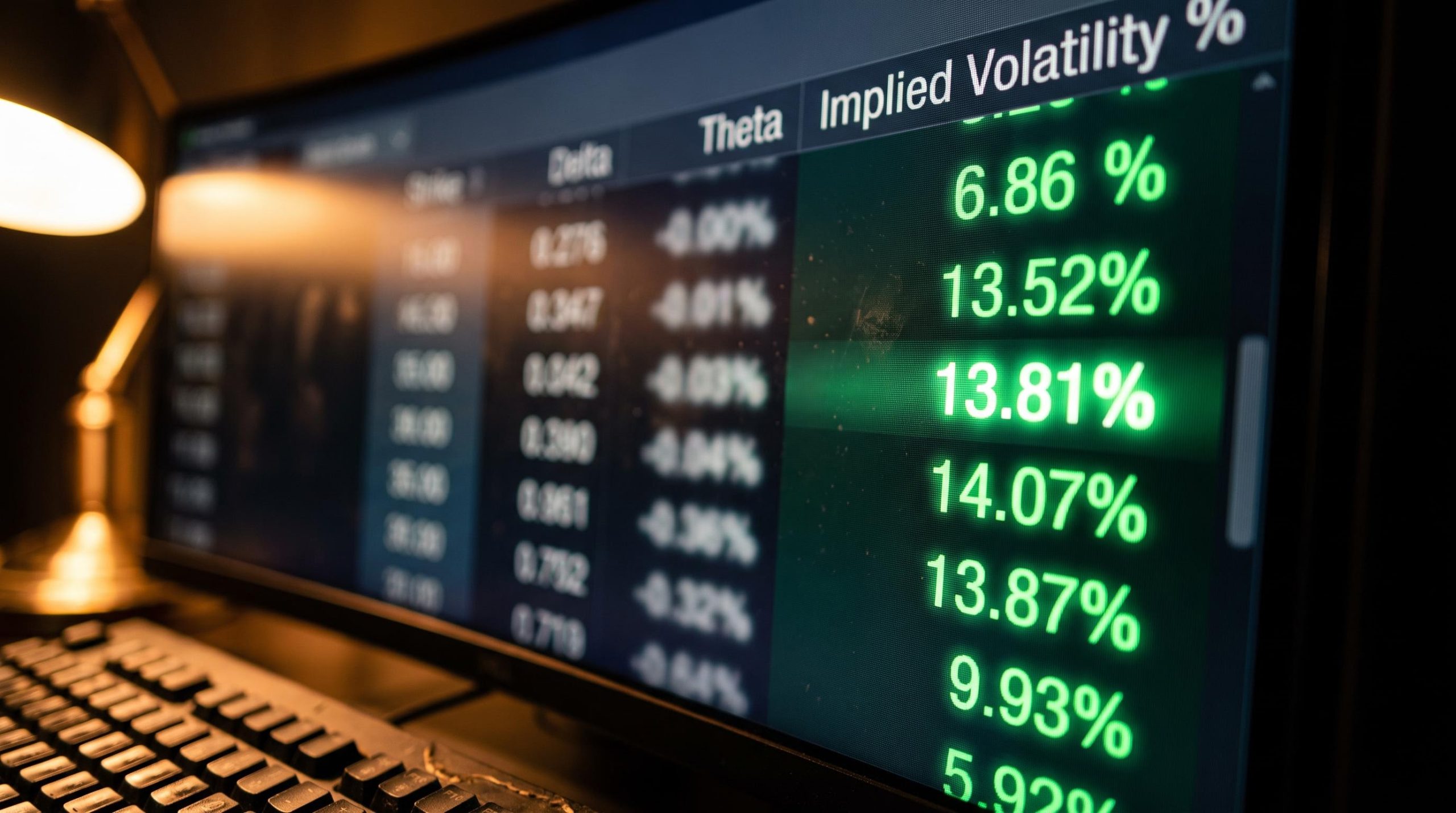
You open an options chain, and there it is: a column of percentages beside every strike price. One reads 13.81%. Another says 30%. They are not prices. They are not Greeks. They sit there without explanation, and if you do not know what they represent, every decision you make from that screen is missing its most important input.
That column is implied volatility, and it is the single number the entire options market uses to express its collective expectation about how much a stock or index is likely to move. Every other figure on the chain, from delta to theta to the probability percentages your platform displays, flows downstream from it. Understanding implied volatility is not an optional refinement for experienced traders. It is the starting point.
Here is what this piece covers: how implied volatility is defined, where the number comes from, why different strikes show different readings, the historical event that permanently reshaped how markets price it, how the Greeks depend on it, and how to use it as a filter for strategy selection. By the end, you will be able to read the IV column on any options chain with genuine comprehension and act on what it tells you.
What implied volatility actually is (and what it is not)
Implied volatility (IV) is the market’s forward-looking estimate of how much an underlying asset’s price is expected to move, expressed as an annualised percentage. More precisely, it represents the annualised standard deviation of expected returns that the options market is currently pricing in.
Core definition: Implied volatility is the annualised percentage standard deviation of expected returns, derived from the current market price of an option, not from historical price data.
That distinction matters. IV is not calculated from what a stock has done in the past. It is extracted from what buyers and sellers are collectively willing to pay for options right now, making it a real-time reflection of market expectation rather than a backward-looking statistic.
The most common and most costly misunderstanding is treating IV as a directional signal. It is not. An IV reading of 30% tells you the market expects a large move. It says nothing about whether that move will be up or down.
Take a broad index versus an individual share. Where the S&P 500 might carry an IV of around 15%, a single equity’s options can reflect something closer to 30%. That difference signals that the market prices in roughly twice the movement for the stock as for the index, but it says nothing about which direction either will travel.
Event-driven IV compression illustrates the principle in practice: options markets priced the July 2026 FOMC at roughly 0.8% implied movement for the S&P 500, approximately 30% below the 1.1% typically embedded before CPI releases, a gap that reflects genuine analytical consensus rather than market complacency.
IV also solves a comparison problem. A $3 option on a $50 stock represents a very different risk profile from a $3 option on a $500 stock. IV standardises those prices into a percentage, making risk comparable across any symbol and any expiration.
Before you enter any options position, the IV reading is the fastest way to calibrate how much movement the market collectively expects. Ignoring it means entering without that calibration.
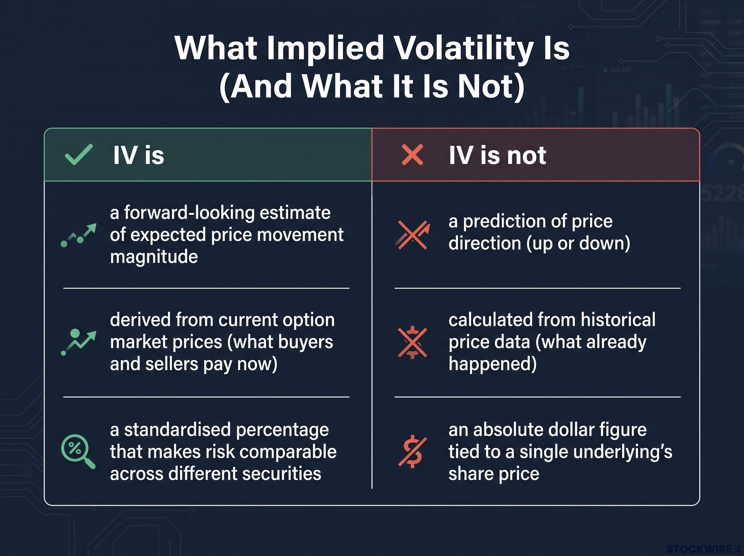
- IV is: a forward-looking estimate of expected price movement magnitude
- IV is not: a prediction of price direction (up or down)
- IV is: derived from current option market prices (what buyers and sellers pay now)
- IV is not: calculated from historical price data (what already happened)
- IV is: a standardised percentage that makes risk comparable across different securities
- IV is not: an absolute dollar figure tied to a single underlying’s share price
When big ASX news breaks, our subscribers know first
How the market price of an option becomes an IV number
The number you see in the IV column is not set by any person, committee, or exchange. It is extracted from the price the market is already showing you.
The process starts with the Black-Scholes options pricing model, which is the standard mathematical framework for calculating what an option should theoretically cost. Its required inputs include the underlying asset’s current price, the option’s strike price, time remaining to expiration, the prevailing risk-free interest rate, and expected dividends. Feed those inputs into the model and it returns a theoretical price. All of those inputs are observable, except one: volatility.
Here is where IV emerges. Instead of plugging in a volatility figure to get a price, traders reverse the process:
- Observe the option’s actual market price (what buyers and sellers have agreed to pay)
- Identify all the known inputs (underlying price, strike, time to expiration, risk-free rate, dividends)
- Back-solve through the pricing model to find the volatility value that makes the model’s theoretical price match the market price
- The result is the implied volatility at that strike
That reverse-engineering runs continuously. Every time the market price of an option shifts, the IV reading updates to reflect the new price.
Looking at the SPX options chain as an illustration: the 7680 strike put had a bid-ask spread of $0.90 to $1.00 and an IV of 13.81%, meaning that plugging 13.81% into the pricing model produces a theoretical value of around $1.07, sitting squarely within that spread. At the 7675 strike, the IV of 14.53% generates a theoretical value of approximately $0.72. Those IV figures were not assigned by anyone; they are simply what the mathematics implies once buyers and sellers set their prices.
Why supply and demand shape the IV reading
When heavy buying pressure pushes an option’s market price higher, the IV extracted from that price rises as a direct consequence. The model’s equation has not changed; the input price has.
This is why IV tends to spike during periods of market stress. Fear-driven buying of protective puts pushes their prices higher, and since IV is extracted from price, the IV reading climbs. A sudden spike in IV on a specific strike is a direct signal of where demand for protection or speculation has concentrated, which is information you can act on.
Fear-driven demand spikes in options markets do not occur in isolation: the same emotional dynamics that push traders toward panic selling in equity markets simultaneously push protective put premiums higher, creating the IV surge that the options chain registers as a sudden rise in strike-specific volatility readings.
Strike-by-strike IV differences and the shape of the skew curve
If you have followed the logic so far, something should puzzle you. If the underlying asset has one expected volatility, why do different strikes on the same expiration show different IV numbers?
In a theoretical Black-Scholes world, they would not. All strikes on the same expiration would carry identical IV. Real markets do not work that way, because each strike has its own market price shaped by its own buyers and sellers. The IV extracted from the 7680 strike reflects different supply-demand dynamics than the IV extracted from the 7710 strike, even though both are options on the same underlying with the same expiration.
Plotting IV against strike price produces a curve rather than a horizontal line, and that curve is what practitioners call the volatility skew. For equity index options such as those on the S&P 500, the curve typically sits lowest near at-the-money (ATM) strikes and slopes upward on both sides, with the rise being considerably steeper toward lower, out-of-the-money (OTM) put strikes than toward higher OTM call strikes. This lopsided shape is often referred to as a volatility smirk.
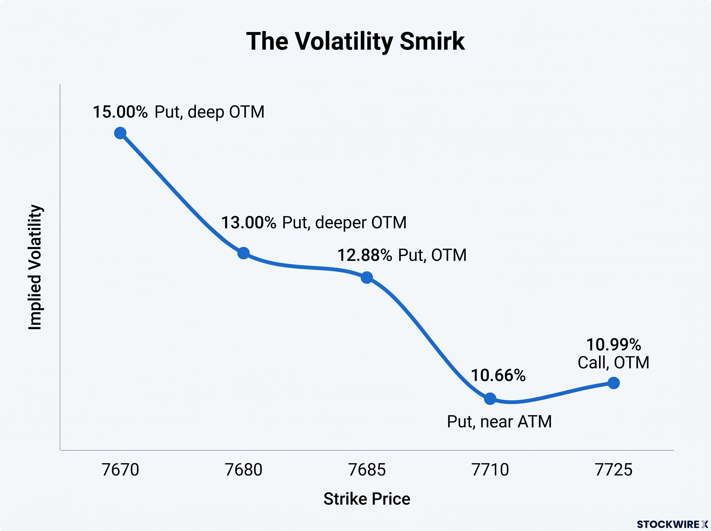
| Strike | Option type | Implied volatility |
|---|---|---|
| 7710 | Put (near ATM) | 10.66% |
| 7685 | Put (OTM) | 12.88% |
| 7680 | Put (deeper OTM) | 13.00% |
| 7670 | Put (deep OTM) | 15.00% |
| 7725 | Call (OTM) | 10.99% |
The pattern is clear. As put strikes move further below the current price, IV rises sharply. On the call side, IV also rises as strikes move higher, but the slope is gentler. When traders collectively anticipate potential downside risk, they bid up the price of OTM puts to secure protection. That elevated demand inflates those options’ market prices, and since IV is extracted from price, it lifts their IV readings with it, creating the steeper slope on the put side of the curve.
Key interpretive point: A steep downside skew signals strong demand for tail-risk protection. It does not predict that a decline will occur.
For you, the steepness of the skew on any given day tells you how much of a premium the market is charging for downside protection. That directly affects the cost-efficiency of buying puts versus the premium available from selling them. A trader who compares IV readings across strikes without understanding that each measures something different will misprice spreads and misinterpret why put premiums cost more than call premiums at equivalent distances from the money.
How a single crash permanently restructured options pricing
Prior to October 1987, the standard practice across options markets was to apply one uniform volatility assumption to every strike within a given expiration. The approach was internally consistent with Black-Scholes theory, but it proved to be a fundamental misreading of how extreme downside risk actually behaves.
What happened next exposed that misreading in the most costly way possible. The sudden, violent market decline revealed that deep OTM index puts had been chronically underpriced: the probability of extreme downside moves was far higher than a single flat volatility assumption implied, and sellers who had written those puts at artificially low premiums faced devastating losses almost overnight. The entire framework for pricing risk across the strike spectrum was invalidated in a matter of hours.
The structural response was immediate and lasting. Post-crash, markets permanently re-priced downside tail risk. OTM puts began trading at persistently higher IV than ATM options, and the volatility smirk became a permanent feature of equity index options. Empirical studies confirmed the shift: short-maturity, deep OTM S&P 500 puts consistently traded at much higher IVs than ATM options, producing the persistent smirk pattern visible in the SPX data above.
NBER research on post-crash S&P 500 options pricing confirmed that short-maturity, deep OTM S&P 500 puts consistently traded at substantially higher implied volatilities than ATM options following 1987, establishing the smirk as a durable structural feature rather than a temporary market anomaly.
Computing infrastructure developed in parallel with this shift. Generating and updating strike-specific volatility figures across a full options chain was a calculation-intensive task, and the processing capacity required to do it reliably only became widely accessible in the years after 1987. The two developments, the market’s new approach to pricing skew and the hardware capable of tracking it, advanced together.
- Pre-1987: A single flat volatility figure was used across all strikes, assuming tail risk was symmetrical and modest
- Post-1987: OTM puts permanently re-priced to reflect the real probability of extreme downside moves
- Pre-1987: Deep OTM puts were systematically underpriced, exposing sellers to catastrophic loss
- Post-1987: The volatility smirk became a durable, structural feature of equity index options markets
The 1987 origin story tells you that skew is not a quirk or an anomaly waiting to be arbitraged away. It is the market’s hard-won adjustment to a reality the original pricing model did not account for. The underlying tail risk it prices is real, which is why skew persists decades later.
Greeks and probability estimates as downstream outputs of IV
All of the derived figures your options chain displays, including delta, gamma, theta, vega, and the probability percentages shown by your platform, are model outputs that each depend on the implied volatility at the specific strike being evaluated. Adjust that IV input, and every downstream figure adjusts with it.
Here is how each major Greek connects back to IV:
- Delta: Measures how much an option’s price changes for a one-point move in the underlying. Its value depends on both moneyness and the volatility assumption at that strike.
- Gamma: Measures how quickly delta itself changes. Higher IV generally increases gamma for near-ATM options, making them more sensitive to small moves.
- Theta: Measures time decay, how much value an option loses per day. Looking at 30-day expiration contracts, the 7675 strike put carries a theta of -$1.57, a figure that is generated using a volatility input of 13.09%. The time-decay reading is itself a function of IV.
- Vega: Measures direct sensitivity to changes in IV. Options with higher vega see larger price changes when IV moves, making vega exposure the primary risk factor for positions held across periods where IV is likely to shift.
What probability estimates on your platform are actually telling you
When your platform shows the likelihood of an option expiring in or out of the money, that figure is a model calculation driven by the IV at the relevant strike. The model applies that volatility input to an assumed return distribution (typically lognormal) and derives a probability from it accordingly. As a concrete example, the out-of-the-money probability displayed for the 7695 strike put is computed using a 11.5% volatility figure drawn from the current market price of that option.
If the IV at that strike shifts because of changing supply-demand conditions, the probability estimate updates automatically. It is always a downstream output of the current IV, not an independent empirical frequency or a guarantee of any outcome.
Every number you use to size a position, set a stop, or evaluate a spread is a model output derived from the current IV at that strike. If IV moves, all those numbers move with it. Treating them as fixed while IV is shifting means you are carrying risk you have not accounted for.
Using IV levels to guide strategy selection
Understanding what IV is and where it comes from gives you a practical first filter: the IV regime your target asset is currently in should shape which strategies you even consider, before direction, before catalyst timing, and before any other variable.
The core principle is relative, not absolute. “High” and “low” IV are always measured against the asset’s own historical range. An IV of 25% might be elevated for a broad index but below average for a volatile biotech stock. The VIX, which tracks S&P 500 implied volatility, serves as a widely recognised benchmark for index-level IV, but every individual asset has its own history to compare against.
IV is relative to an asset’s own history, not to absolute numbers or cross-asset benchmarks. An IV reading only becomes actionable when you know where it sits within the range that asset has historically occupied.
Elevated IV relative to an asset’s historical range makes premium-selling strategies more compelling, because the premiums available tend to exceed the movement that ultimately occurs. Conversely, when IV sits in the lower portion of its historical range, buying premium becomes more attractive: options are cheaper, and any subsequent expansion in volatility or a large directional move can deliver a favourable return.
Credit spreads are among the most frequently selected high-IV strategies because positive theta aligns the trader with time rather than against it: each day that passes without a large adverse move adds to the position’s profit, making them structurally suited to environments where IV is elevated relative to what the market ultimately realises.
| High-IV strategies (selling premium) | Low-IV strategies (buying premium) |
|---|---|
| Selling covered calls | Buying long calls or puts |
| Writing cash-secured puts | Constructing debit spreads |
| Credit spreads | Pre-catalyst straddles |
| Iron condors | Pre-catalyst strangles |
The IV regime is your opening filter. Look up the current IV for any asset you trade, compare it to its historical range, and use that comparison as the first step before selecting a strategy. Direction and catalyst timing come second.
Past performance does not guarantee future results. The tendency for implied volatility to overstate realised volatility is a historical pattern, not a guaranteed outcome.
Reading IV as a risk language, not a crystal ball
Everything in this piece connects to a single reframe. Implied volatility is not a mysterious number to scroll past on the options chain. It is the language the market uses to express its collective expectation about risk, and your job as a trader is to read it fluently.
The thread runs through every section. IV is extracted from market prices, not imposed on them. Skew maps where that expectation concentrates along the strike spectrum. The Greeks and probability estimates flow from it. Strategy selection begins by reading it correctly.
The boundary remains firm: IV reveals expected magnitude of movement and where hedging demand sits. It cannot predict direction. It cannot guarantee outcomes. Treating it as a calibration tool rather than a forecast allows you to align your risk exposure with what the market is genuinely pricing, rather than what you might wish it were pricing.
Strategy expectancy captures the mathematical dimension that IV regime analysis cannot: even a correctly identified high-IV environment does not guarantee that a premium-selling approach produces a net-positive result unless the win rate and average payoff size combine to produce a positive expected value across a meaningful sample of trades.
A trader who reads IV fluently enters every options position with the market’s own risk assessment already translated. You know what the price implies about expected movement, where hedging demand sits along the strike spectrum, and whether the current environment favours collecting premium or spending it. That is not a prediction. It is preparation.
IV is a calibration tool, not a forecast. It tells you how much, not which way. Read it for what it is, and every other decision on the options chain becomes more informed.
This article is for informational purposes only and should not be considered financial advice. Investors should conduct their own research and consult with financial professionals before making investment decisions.