How to Control Portfolio Risk Before the Next Market Shock

A portfolio split equally between a technology ETF and a utilities ETF looks balanced on a brokerage statement. In risk terms, the technology side carries roughly nine times more market exposure than the utilities side. Most investors have never run this calculation, and the gap between dollar allocation and risk allocation goes unnoticed until a market shock makes it unmistakable. When the VIX spiked from the mid-teens to above 80 during March 2020, portfolios that appeared diversified on paper delivered drawdowns their owners never intended to take. This guide walks through two rules-based frameworks, beta-weighted position sizing and volatility targeting, that together give investors deliberate, measurable control over how much risk a portfolio actually carries. Concrete numerical examples throughout make each step replicable at the next rebalancing date.

Why your portfolio’s dollar split tells you almost nothing about its actual risk

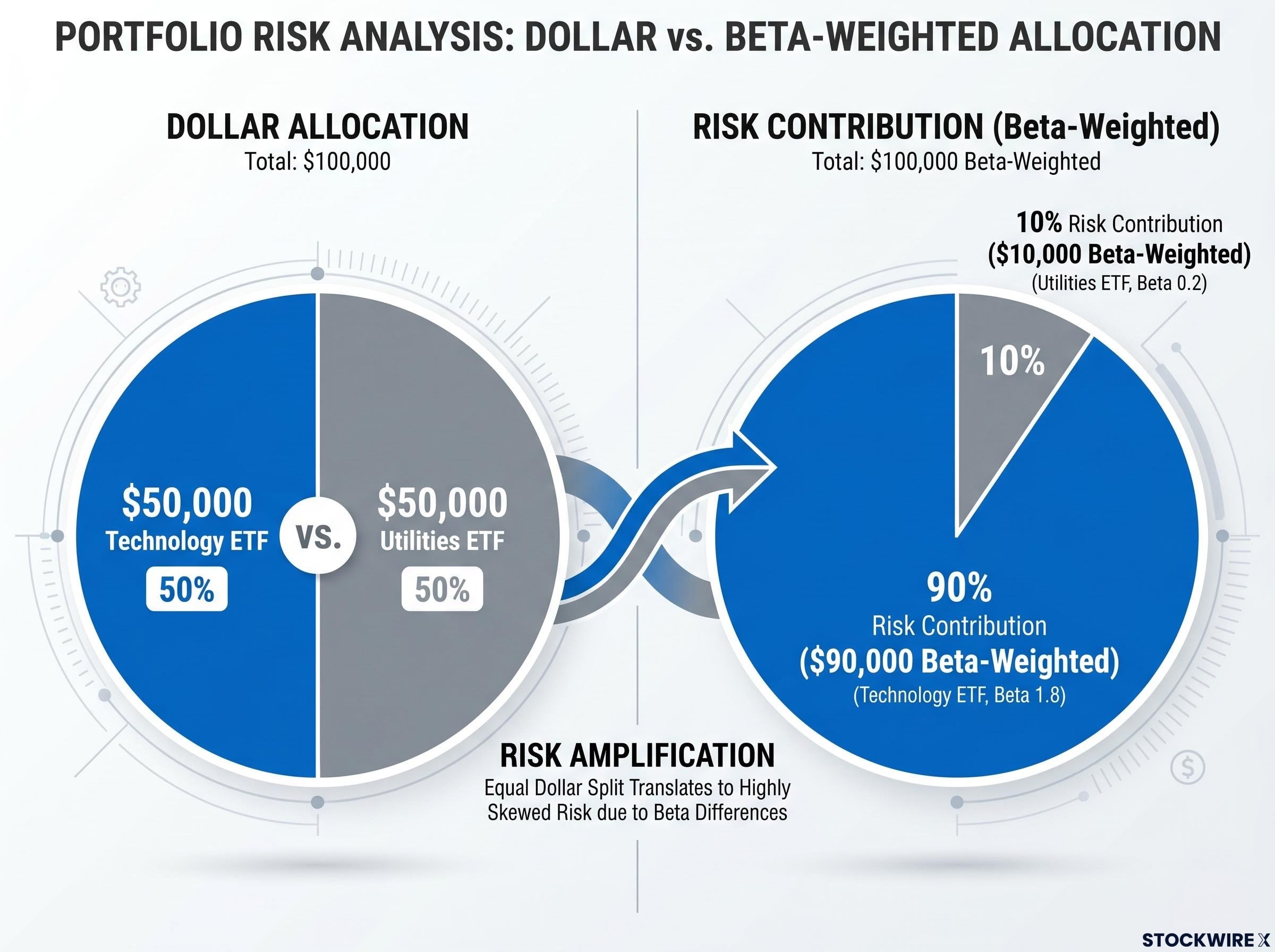
Consider a $100,000 portfolio divided equally: $50,000 in a technology sector ETF with a beta of approximately 1.8, and $50,000 in a utilities ETF with a beta of approximately 0.2. The brokerage statement shows a clean 50/50 split. The risk contribution tells a different story.

Beta-weighted dollars convert each position’s dollar size into its market-risk equivalent by multiplying the dollar allocation by the position’s beta. For the technology ETF, that calculation is $50,000 x 1.8 = $90,000 in beta-weighted terms. For the utilities ETF, it is $50,000 x 0.2 = $10,000.

The risk split: approximately 90% of this portfolio’s market-risk contribution comes from the technology position, and just 10% from utilities, despite identical dollar sizes.

The beta values used here are illustrative and regime-dependent, not permanent point estimates. But the underlying principle holds regardless of the specific numbers: equal dollar weights do not produce equal risk weights, and the gap can be extreme. Investors who see this calculation for the first time often realise their portfolio has been far more aggressive than intended for years.

High-beta equity drawdowns can be factor-specific rather than broad market events, as the June 2026 momentum unwind demonstrated: high-beta momentum equities fell approximately 9.5-10% in a single session while the S&P 500 remained up over 10% year-to-date, isolating the damage almost entirely within overweight positions carrying elevated beta exposure.

Beta explained: what the number actually measures (and what it misses)

Beta measures how much an asset’s price tends to move relative to a benchmark, with the S&P 500 conventionally set at 1.0. A stock with a beta of 0.5 is expected to move roughly 5% for every 10% market move, tracking direction but with reduced amplitude. A beta of 1.8 amplifies in both directions, meaning a 10% decline in the benchmark corresponds to roughly an 18% decline in the position.

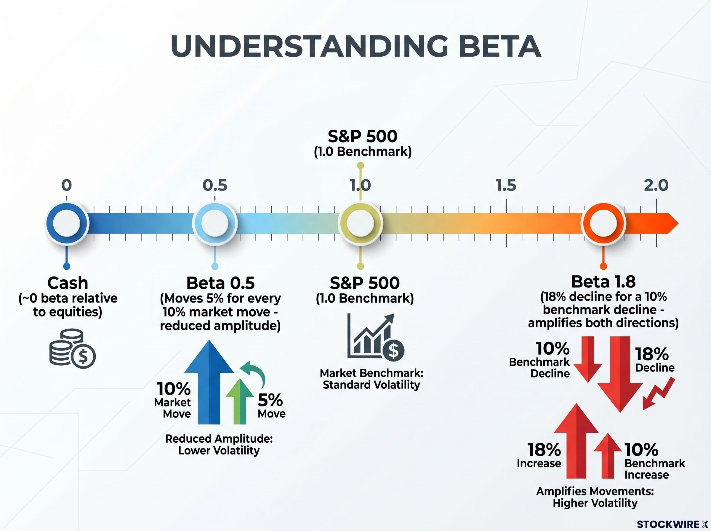
Beta is not the same thing as correlation. Correlation measures whether two assets move in the same direction; beta incorporates both correlation and relative volatility simultaneously, making it a richer measure but also a more unstable one. Cash carries a beta of approximately zero relative to equities but still exposes holders to inflation erosion. Assets with negative beta, such as long-duration Treasuries, can shift toward positive beta when inflation expectations dominate, as occurred in periods when bonds and equities fell together.

Value investors define risk as the probability of permanent capital loss rather than price volatility or beta, a philosophical inversion that produces fundamentally different portfolio construction logic: where beta weighting starts from market sensitivity, margin of safety analysis starts from business quality and discount to intrinsic value.

Where beta estimates come from and why they differ

Different financial data providers report different betas for the same ETF. The variation comes from three inputs:

• Lookback period: A 1-year beta captures recent regime behaviour; a 5-year beta smooths across multiple conditions.
• Return frequency: Daily returns produce different estimates than weekly returns.
• Benchmark choice: An ETF’s beta relative to the S&P 500 will differ from its beta relative to a global index.

The practical rule is consistency. When computing portfolio beta, pull all position betas from the same source using the same methodology to avoid mixing incompatible estimates.

What beta does not capture matters just as much as what it does:

• Idiosyncratic sector risks (regulatory changes, patent cliffs, supply chain disruptions)
• Inflation risk embedded in cash positions
• Duration risk in bond holdings
• Crisis correlation convergence, where assets that appeared uncorrelated under calm conditions decline simultaneously during liquidity events

Beta is a steering tool, not a precision instrument. Investors who understand its limits will use it deliberately rather than over-trust it.

How to size positions using beta to set your intended risk exposure

The portfolio beta formula translates the risk contribution problem into arithmetic investors can act on:

Portfolio beta = sum of (weight x beta) across all positions

Applied to the two-ETF example at a 65/35 split:

(0.65 x 1.8) + (0.35 x 0.2) = 1.17 + 0.07 = 1.24

A 65% technology / 35% utilities allocation produces a portfolio beta of approximately 1.24, meaning the portfolio is expected to move roughly 12.4% for every 10% move in the S&P 500.

The steps to apply beta-weighted sizing are straightforward:

1. List all positions with their current dollar values and betas (pulled from a consistent source).
2. Compute each position’s beta-weighted dollar contribution (dollar value x beta).
3. Sum the beta-weighted contributions to calculate total portfolio beta.
4. Compare the result to a target beta that reflects the intended risk profile.
5. Adjust position weights until portfolio beta and individual risk contributions align with the target.

A practical diversification cross-check: consider limiting any single sector or theme to a maximum of approximately 20-30% of total portfolio risk contribution, not just 20-30% of dollar allocation. The two thresholds produce very different portfolios when position betas diverge significantly.

To equalise beta-weighted risk contributions in the original example, roughly $90,000 would need to go to utilities and only $10,000 to technology, given the ninefold difference in beta per dollar invested. That allocation looks absurd by dollar weight, but it is what equal risk contribution actually requires.

Beta weighting does not demand equal risk across all positions. It ensures that whatever risk distribution exists is the result of a conscious decision rather than an accidental artefact of dollar sizing.

Risk-balanced construction taken to its logical extreme is the foundation of Ray Dalio’s All Weather approach, which allocates across four economic quadrants rather than across asset-class labels, with each quadrant weighted by its risk contribution rather than its dollar share, producing a portfolio where no single macro regime dominates total drawdown exposure.

Using volatility targets to manage portfolio risk

Beta weighting sets the risk structure of a portfolio: how sensitive each dollar is to benchmark moves. Volatility targeting addresses a different dimension, risk magnitude, meaning the absolute size of the portfolio’s price swings over time. A portfolio can have a deliberate beta structure and still experience swings far larger than intended if market volatility itself spikes. The two frameworks are complementary, not overlapping.

NBER research on volatility-managed portfolios finds that scaling equity exposure inversely with realized variance produces significant improvements in risk-adjusted returns across multiple asset classes, providing academic backing for the mechanical scaling approach described here.

Choosing a volatility target that fits your risk profile

Annualised volatility targets generally fall into three tiers:

• Conservative (retired investors or those with low risk tolerance): 5-10% annualised volatility
• Moderate: 10-15% annualised volatility
• Aggressive: 20-25% annualised volatility, corresponding to significantly larger portfolio swings

Realised volatility is typically estimated using 6-12 months of daily returns, annualised, as the input to the scaling formula. Monthly or quarterly monitoring is a reasonable schedule. Adjusting only when realised volatility deviates more than approximately 20-30% from the target avoids overtrading on noise.

The scaling formula is:

New risky weight = Current risky weight x (Target volatility / Current volatility)

Two scenarios illustrate how it works in practice:

When the scaling factor rises above 1.0, institutional strategies may use leverage to increase total exposure. For individual investors, the adjustment mechanism is a cash or short-duration Treasury ETF buffer rather than leverage. When volatility compresses, the buffer shrinks in favour of risky positions; when volatility spikes, the buffer grows.

During March 2020, the VIX rose from the mid-teens to above 80 in roughly three weeks. Portfolios calibrated to any volatility target experienced two to three times their intended exposure during the spike. A volatility-targeting framework is designed to detect and respond to such regime shifts, though with any backward-looking estimate, there is an inherent lag before the signal fully reflects the new environment.

Putting the two frameworks together: a repeatable rebalancing process

The practical payoff of combining beta weighting and volatility targeting is a single integrated workflow that checks both the shape and the magnitude of risk in each rebalancing cycle. The following six steps form that workflow:

1. List all positions with current market values.
2. Pull betas from a consistent source (same lookback period, same benchmark across all positions) and compute portfolio beta plus each position’s beta-weighted dollar contribution.
3. Adjust allocations to reach the target portfolio beta with no single sector or theme exceeding 20-30% of total risk contribution.
4. Estimate realised volatility of the overall portfolio using 6-12 months of daily returns, annualised.
5. Apply the scaling formula (new risky weight = current risky weight x (target volatility / current volatility)) and allocate the remainder to cash or short-duration Treasury ETFs.
6. Re-check both dimensions on a monthly or quarterly schedule, adjusting when realised volatility deviates more than 20-30% from the target.

Steps 2 and 4 require the same discipline: a consistent methodology applied each time. Switching data sources or lookback windows between rebalancing cycles introduces noise that has nothing to do with actual portfolio risk changes.

The goal is keeping risk within a reasonable band, not hitting precise decimal-point targets. Beta and volatility estimates are steering tools. Treat targets as directional guides rather than exact values to match.

The monthly or quarterly re-check is where both frameworks converge. At that moment, the investor confirms that risk structure (the beta-weighted contribution of each position) and risk magnitude (the portfolio’s realised volatility relative to target) are both within their intended bands simultaneously. If either has drifted beyond the threshold, the six-step sequence identifies where to adjust.

The honest limits of both tools, and why they still matter

Every estimate used in these frameworks, beta, realised volatility, correlation, is backward-looking. These numbers reflect what the portfolio looked like over the measurement window, not what it will look like in the next regime shift. They will be wrong at precisely the moment they are most needed.

The specific failure modes are worth stating directly:

• Beta instability under stress: During liquidity crises, asset correlations converge toward one. Positions that appeared diversified under calm conditions decline together, as occurred during both the 2008 global financial crisis and the March 2020 market disruption.
• Volatility estimation lag: Backward-looking realised volatility inherently lags a sudden regime shift. When the VIX moved from the mid-teens to above 80 in roughly three weeks during March 2020, any rolling estimate took time to reflect the new environment.
• Sector concentration blindspot: Beta arithmetic cannot reveal that three different ETFs in a portfolio all hold concentrated positions in the same underlying companies or themes. Examining underlying holdings is necessary to detect unintentional exposure doubling.

None of these limitations makes the frameworks useless. They make the frameworks imperfect, which is a different claim.

The value proposition, stated honestly: beta weighting and volatility targeting do not eliminate risk surprises. They reduce the probability of large, unintentional mismatches between the risk an investor intends to carry and the risk the portfolio actually contains. A portfolio built by dollar weight alone has no mechanism to detect such mismatches. A portfolio built with these tools has one.

Readers who understand these limits will maintain the monitoring discipline the frameworks require, rather than setting a target once and assuming it holds indefinitely.

This article is for informational purposes only and should not be considered financial advice. Investors should conduct their own research and consult with financial professionals before making investment decisions. Past performance does not guarantee future results, and all estimates described here are backward-looking and subject to change under shifting market conditions.

Risk is a design choice, not a discovery

The gap between perceived risk and actual risk exposure is not inevitable. It is a product of building portfolios by dollar weight rather than by risk weight. Beta weighting sets the risk structure deliberately, ensuring each position’s contribution to total portfolio risk reflects a conscious decision. Volatility targeting keeps the risk magnitude within the intended envelope as market conditions shift, scaling exposure mechanically rather than emotionally.

Together, these frameworks convert portfolio risk from something investors discover during a drawdown into something they design in advance and monitor systematically.

The next step is concrete: run the beta-weighted calculation on a current portfolio before the next rebalancing date. Compare each position’s risk contribution percentage to what was intended. If the numbers diverge, the tools to close the gap are now in hand.

For investors ready to put the six-step framework into action at the next rebalancing date, our full guide to portfolio rebalancing execution covers the specific sequencing decisions: when to use new contributions versus sales, how to handle tax-advantaged versus taxable accounts, and which alternative asset classes offer lower correlation for reallocated capital.