Most income investors work from a simple rule: to benefit from an asset’s distributions, you hold it. Covered call ETFs quietly break that assumption. Their distribution mechanics create a specific structural window where a short-term position can, in theory, capture the payout without a long-term commitment.
That window matters more now than it used to. In a rate-plateau environment, investors hunting for yield are looking past conventional dividend stocks toward structured income products, and covered call ETFs sit at the intersection of options income and equity exposure. That combination makes their distributions unusual enough to support a timing-based approach that simply does not work on ordinary shares.
The catch is that this is one of the most misunderstood corners of income investing, and the mechanics that make it interesting are the same ones that make it dangerous. What follows is a clear breakdown of how the strategy is constructed, where it can work, and where it falls apart, so you can judge whether the arithmetic actually holds before committing any capital.
Why covered call ETF distributions are not like ordinary dividends
If you have ever considered dividend capture, buying a stock just before its ex-dividend date to collect the payout, you already know the logic. You also know why it rarely works: the share price drops by roughly the dividend amount on the ex-date, so you are not collecting free money, you are betting on a quick recovery.
Covered call ETF distributions look similar on the surface. Underneath, they are a different animal entirely.
An ordinary stock dividend is a single, transparent thing: cash paid out of company earnings. Its ex-date price drop is predictable, and its source is obvious. A covered call ETF distribution is a blend of three separate sources:
The covered call ETF income mechanics that produce those high headline yields involve a permanent structural trade-off: the fund sells call options on its holdings to collect premium, which caps the price upside the underlying equities would otherwise deliver to unitholders.
- Option premiums: income collected from selling call options on the fund’s holdings. This is not tied to the fund’s underlying asset value the way earnings are.
- Ordinary dividends: the regular dividends paid by the equities the fund actually holds.
- Return of capital or realised gains: realised capital gains, losses, or a return of the investor’s own principal.
That third source is where the trouble hides.
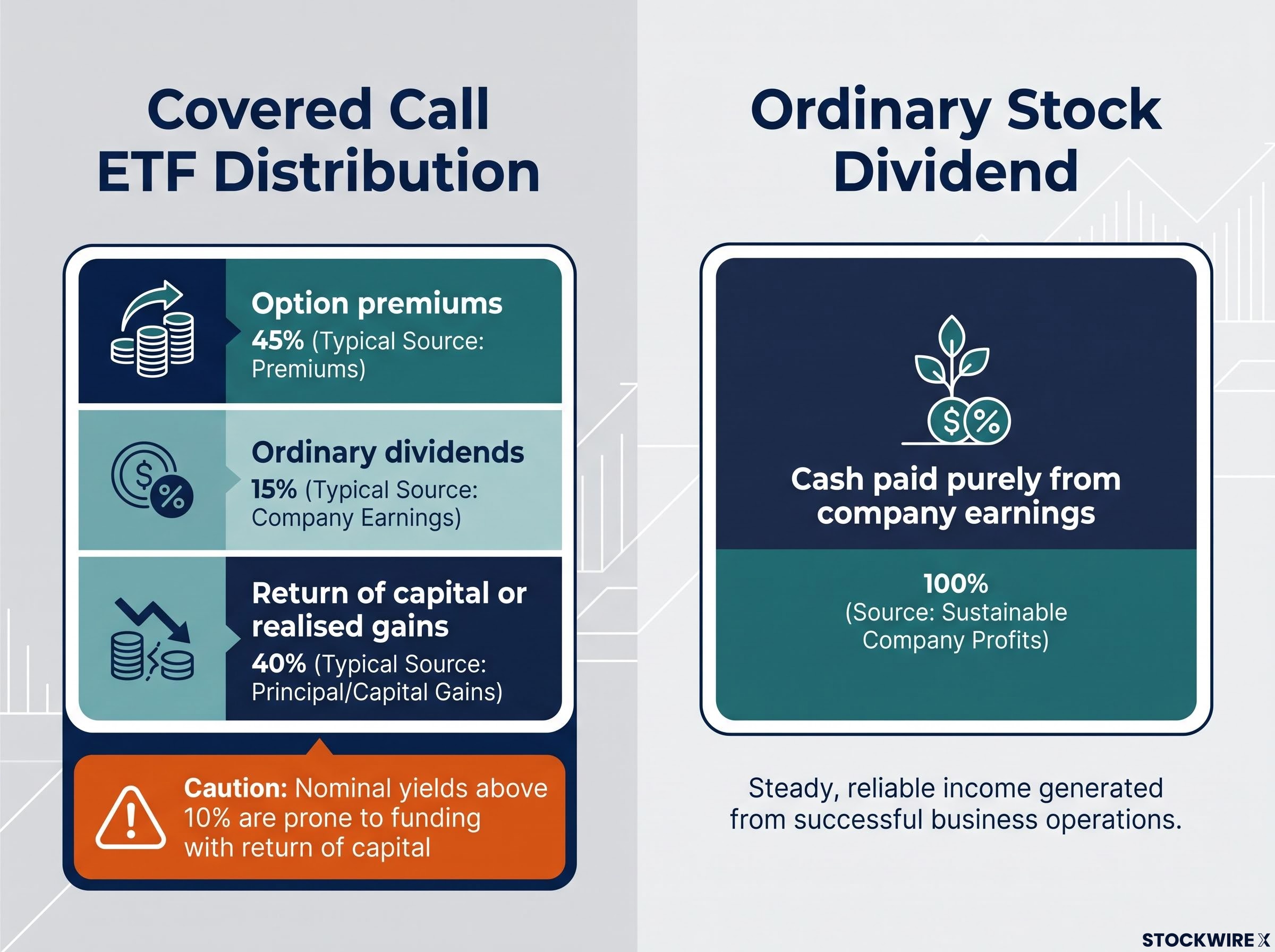
Key caution: high yields often mean your own money back High-yield covered call ETFs targeting nominal yields above 10% are especially prone to funding distributions with return of capital. That portion does not represent earned income. It is your own principal being handed back to you, dressed up as yield.
Because part of the distribution is option premium, and because covered call structures cap upside by selling calls, the fund sacrifices capital appreciation to generate that premium. That trade-off changes how the net asset value (NAV), the per-unit value of the fund’s holdings, behaves relative to what it pays out. The recovery dynamics after an ex-date behave differently from a standard dividend stock.
For you, the practical implication is direct: the headline yield on a covered call ETF is not a pure income number the way a bond coupon or savings rate is. Part of it may be your own money coming back to you, and knowing that before you enter any short-term position is the whole game.
| Attribute | Covered call ETF distribution | Ordinary stock dividend |
|---|---|---|
| Income source | Blend of option premiums, dividends, and return of capital or realised gains | Cash paid purely from company earnings |
| Ex-date price drop predictability | Less predictable; recovery shaped by premium mechanics and NAV trend | Predictable; price drops by roughly the dividend amount |
| NAV erosion risk | Elevated in high-yield funds paying more than they earn | Minimal; distribution reflects genuine earnings |
When big ASX news breaks, our subscribers know first
How the income capture strategy works in practice
The mechanics are straightforward enough to follow as a sequence. You take a position shortly before the ex-distribution date, hold through the distribution, and close the position shortly after, rather than holding for long-term appreciation.
Here is the sequence in practice:
- Identify a target covered call ETF with a NAV trend that is not in persistent decline.
- Confirm the ex-distribution date, typically clustered at month-end for monthly-paying funds.
- Enter the position ahead of that date.
- Hold through the ex-date to become eligible for the distribution.
- Monitor the post-distribution price recovery closely.
- Exit the position once the price has recovered enough to leave a net gain.
This is framed as an income capture strategy rather than dividend capture for a specific reason. Covered call ETFs typically pay monthly, not quarterly, which creates a repeatable timing window that individual dividend stocks simply do not offer. Leading Canadian covered call funds illustrate the product category well: the BMO Covered Call Utilities ETF (ZWU) has been reported at an annualised yield near 7.39%, while the Hamilton Enhanced Utilities ETF (HUTS) announced a monthly distribution of $0.0750 per unit. Treat these as illustrations of the category, not recommendations. The specific figures shift with each fund’s distribution announcement.
Where the logic breaks down
The problem is baked into the mechanics. On the ex-distribution date, the ETF’s price mechanically drops by roughly the distribution amount, because the market prices the payout out of the NAV. You are not capturing free income. You are betting the price recovers inside your short holding window, and that recovery is never guaranteed.
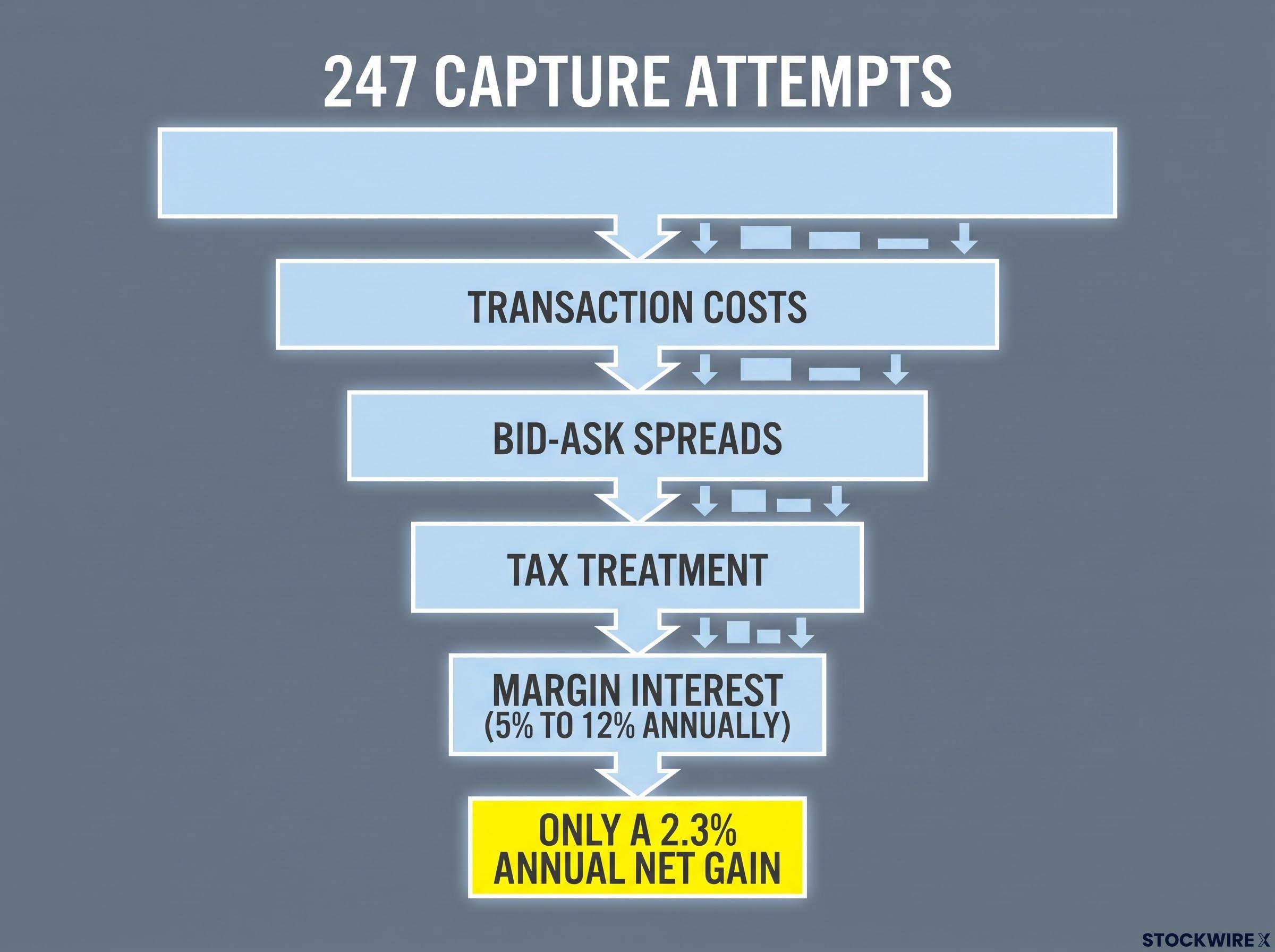
Then the friction layer arrives. Transaction costs, bid-ask spreads (the gap between the price to buy and the price to sell), and tax treatment all chip away at the captured distribution before it becomes net income.
An illustrative reality check One empirical tracking exercise of 247 capture attempts produced only a 2.3% annual net gain. Treat this as illustrative rather than an authoritative institutional study, but it captures the point: the margins are thin once friction is counted.
In high-yield ETFs with persistent NAV erosion, the danger sharpens. If the fund’s NAV is drifting downward because it pays out more than it earns, the post-distribution price may never return to its pre-distribution level, leaving you holding a slowly declining asset.
NAV erosion in high-yield funds follows a specific pattern: distributions paid in excess of earned income reduce the fund’s per-unit value, so the monthly cheque arrives on schedule while the underlying asset quietly declines, a dynamic that can leave investors materially worse off than a lower-yielding but structurally sound alternative.
The strategy’s logic is sound in theory, but it is execution-sensitive in practice. Slippage, spreads, or the ETF’s own NAV trajectory can each, on its own, be enough to turn a promising-looking trade negative.
Using bond yield signals to time entries
This is where disciplined execution parts ways with guessing. Buying blindly ahead of a distribution date is speculation. Adding an interest rate signal gives you an actual reason to believe the ex-date drop will recover.
Start with the observable relationship. Utilities, a common holding in these funds, are widely treated as bond-like equities because they carry heavy debt and pay competitive yields. When bond yields rise, utility ETFs tend to fall, because their income now competes with higher-paying fixed income. When yields fall or plateau, utility ETFs tend to recover.
Bond yield signals carry different interpretive weight depending on what is driving them: a yield decline caused by improving disinflation expectations has different implications for utility equity valuations than one driven by a flight-to-safety bid, and the covered call ETF entry signal described here is most reliable when the rate move reflects the former rather than the latter.
The quantitative anchor Empirical frameworks model utilities as long-duration equities with a beta of roughly 0.2 to 0.3 to interest rate changes. That translates to sector moves of about negative 8% to positive 12% for a 100 basis point shift in long yields.
From rate mechanism to divergence signal
The entry signal is not simply a falling yield. It is a divergence. You watch the 10-year government bond yield for a decline, then check whether the covered call ETF’s price has failed to recover in line with what that yield move would imply. That gap, yields down but the ETF still depressed, is the signal that the fund may be undervalued relative to the rate environment.
As a point-in-time anchor, Canada’s 10-year yield stood near 3.94% to 3.96% in mid-September 2026, the environment in which this strategy is being documented.
| Rate environment condition | Implied signal for income capture |
|---|---|
| Yields rising | Cautious |
| Yields plateauing | Neutral |
| Yields falling, ETF not yet recovered | Entry signal |
| Yields falling, ETF already recovered | Already priced in |
For you, this timing layer is the difference between a thoughtful entry and a hopeful one. The divergence gives you a concrete, observable reason to expect the ex-date drop to reverse.
What rate signals cannot tell you
The signal has limits, and over-reading it is a common error. Rate sensitivity is not uniform: large-cap regulated utilities react differently from renewables or small-cap names. Markets also tend to anticipate rate moves, so the ETF price may already reflect an expected yield change before it actually happens.
The bond yield is one input, not a complete system. Sector fundamentals, the ETF’s own NAV trend, and broader equity conditions are all co-inputs the rate signal cannot replace. Treat it as a necessary condition, not a sufficient one.
Why margin amplifies both the opportunity and the risk
Margin, borrowing from your broker to increase position size, is where this strategy gets its firepower and its danger. The idea is to fund a larger income capture position than your own capital would allow, so the distribution received covers the borrowing cost and still leaves a net yield.
The arithmetic is unforgiving. For a margin-funded capture to generate net income, three things must all be true at once:
- The distribution received exceeds the ex-date price drop that fails to recover.
- Price recovery actually occurs within your short holding window.
- The margin interest cost is covered by whatever distribution remains after the first two.
Now the numbers. Margin interest rates typically run 5% to 12% annually. Even over a holding period of just a few weeks, that interest is a measurable drag against a monthly distribution. This is why the short holding window matters: it limits margin risk, but it does not remove it. That is a deliberate contrast with long-term passive margin exposure, which is currently considered undesirable given prevailing market conditions.
A direct suitability warning Investors who are new to margin, or who feel anxious about their existing holdings, are advised not to use margin strategies until they have built more market experience. This is not a beginner’s tool.
For you, the personal test is simple. If the break-even maths feels uncomfortable to calculate, or the idea of a margin call during your holding window creates anxiety rather than manageable risk awareness, this strategy does not fit your current stage.
The forced liquidation problem
Here is the tail risk that turns a bad week into a serious loss. If the ETF’s price falls enough during your holding window to breach the maintenance margin requirement, the minimum equity your broker demands, the broker can force a sale at the worst possible moment. One forced liquidation can wipe out the gains from several previous capture trades.
This is not hypothetical. The ex-date price drop itself can add to margin pressure if you entered the position close to the maintenance threshold. And equity portfolios have historically faced drawdowns of 10% to 20% roughly once a decade, any of which could land squarely inside a capture window and trigger exactly this scenario.
Margin debt risk signals at the macro level reinforce the individual position-sizing discipline the suitability checklist describes: with US margin balances at record levels and both Leuthold Group warning thresholds simultaneously breached, any leveraged holding window that overlaps with a broad market correction faces amplified forced-liquidation pressure beyond what fund-specific NAV trends alone would suggest.
Assessing whether the trade makes sense before you enter
By now the pieces are on the table, so here is the practical part: a checklist to run before you commit capital. Work through it in order.
- Confirm the yield divergence. Are bond yields declining while the ETF has failed to recover? Without that gap, you have no rate-based reason to expect the ex-date drop to reverse.
- Assess the NAV trend. Is the fund’s NAV stable, or drifting persistently downward? A declining NAV means the price may never return to your entry level.
- Review the distribution composition. Is the payout weighted toward option premium and genuine dividends, or heavy with return of capital? The former is earned income. The latter is your own principal.
- Calculate the margin break-even. Does the expected distribution clearly exceed borrowing cost plus recovery risk before friction? If the number is marginal, the trade probably does not survive real-world slippage.
- Assess the holding-window risk. Could a market dislocation during your holding period trigger a margin call? Size the position with that scenario in mind.
- Consider buy-and-hold instead. Would simply holding the ETF through multiple distribution cycles serve you better?
That last point deserves emphasis. For most investors, holding a quality covered call ETF through multiple cycles will outperform short-term capture once transaction costs, tax treatment, and unfavourable holding windows are counted. Buy-and-hold benefits from capital gains deferral and compounding, both of which short-term capture structurally forfeits.
The strategy is more defensible in low-friction environments, tight spreads, low brokerage, favourable tax treatment in your jurisdiction, and less defensible as friction climbs. It is also worth noting that funds yielding 7% to 9% may offer a cleaner capture profile than ultra-high-yield products chasing 12% or more, precisely because those top-end yields tend to carry heavier return-of-capital risk.
This article is for informational purposes only and should not be considered financial advice. Investors should conduct their own research and consult with financial professionals before making investment decisions. Past performance does not guarantee future results, and these figures are illustrative and subject to change with market conditions.
Not every investor who finds this strategy intellectually interesting is the right investor to execute it. The checklist exists to surface that gap before your capital is at stake.
What the strategy is, and what it is not
For a financially experienced, margin-capable investor who actively monitors rate signals and ETF NAV trends, income capture on covered call ETFs offers a structured approach to short-term yield generation. It is mechanically distinct from speculation, and it is not the same as chasing dividends on ordinary shares.
It is not a passive income machine. Ex-date price drops, NAV erosion in high-yield funds, margin interest costs, and transaction friction all work against you. Producing a net positive result demands genuine diligence, not a set-and-forget mindset.
And the conditions that make it viable are not fixed. In the mid-September 2026 rate environment in which this strategy is documented, plateauing yields shape the backdrop. As rates shift and covered call ETF structures evolve, the entry conditions will change with them.
That is the real discipline the strategy asks of you: not a one-time judgement, but an ongoing one. The trade that makes sense today may not make sense next month, and the investor who keeps watching bond yields and distribution composition is the one positioned to know the difference.