
For every $1 of available cash sitting in U.S. margin accounts right now, there is roughly $6 to $7 of borrowed money stacked on top of it. That ratio has nearly doubled since late 2023, and it is not a figure you will find in most market commentary. The headline number, margin debt approaching $1.5 trillion, gets the attention. The ratio is what determines how fast things break.
The question worth asking is not whether a correction is coming. Nobody knows that. The question is what happens to the severity of a correction given the leverage architecture currently underneath U.S. equities, and what happens when the most crowded trade in a generation, semiconductors and AI, sits at the centre of that architecture.
Here is the framework for stress-testing whether your own portfolio is positioned to absorb a sharper-than-expected drawdown, or whether you are closer to being a forced seller than you think.
The leverage architecture behind today’s record margin debt
FINRA reported customer margin debit balances of $1.416 trillion in May 2026, the highest nominal reading in the dataset going back to 1997. By June 2026, that figure had risen further to approximately $1.50-$1.53 trillion. Year-over-year growth stood at 53.7% as of May.
Both Leuthold Group warning thresholds have been simultaneously breached for the first time since the dot-com peak: 54% absolute year-over-year margin debt growth and 26% excess growth over market returns, a configuration that preceded average 12-month forward returns of -6.7% across the three prior comparable episodes.
Those are large numbers. They are also the wrong numbers to focus on.
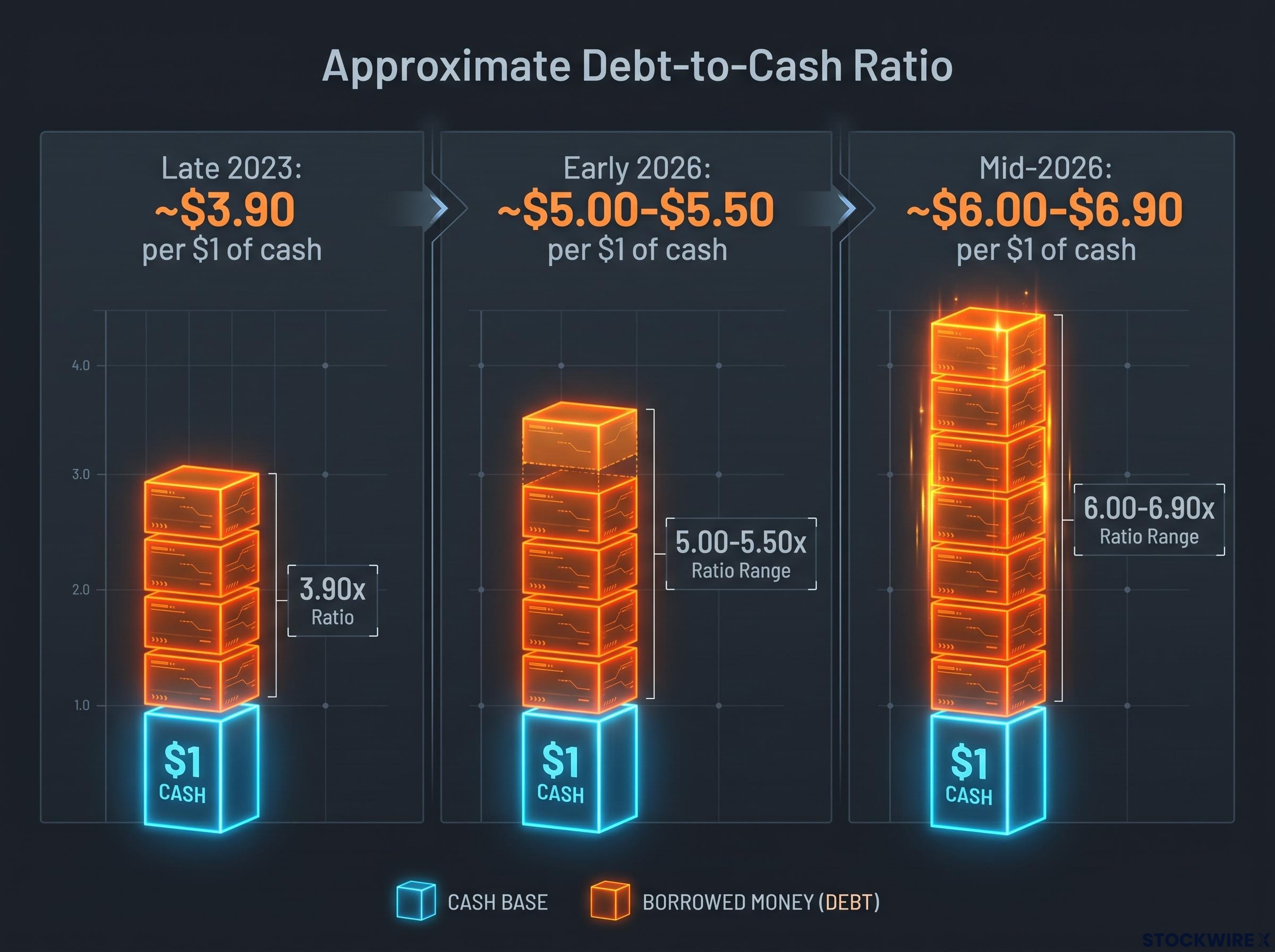
The structural concern lives in the ratio. Free credit balances, the unborrowed cash available across margin and cash accounts, totalled roughly $420-$430 billion against more than $1.4 trillion in margin debt. That produces a debt-to-cash ratio of approximately $6.00-$6.90 of borrowed money for every $1 of available cash, up from roughly $3.90 in late 2023.
| Period | Approximate debt-to-cash ratio |
|---|---|
| Late 2023 | ~$3.90 per $1 of cash |
| Early 2026 | ~$5.00-$5.50 per $1 of cash |
| Mid-2026 | ~$6.00-$6.90 per $1 of cash |
What this tells you is that the market’s current support rests far more on borrowed capital than on fresh investor conviction. The cushion available to absorb price declines before forced selling begins is historically thin.
From headline debt to net investor position
The clearest single expression of this fragility is the net investor credit balance, which is approaching negative $1 trillion. In plain terms, margin borrowers collectively owe nearly $1 trillion more than they hold in available cash across their accounts.
The absolute debt figure tells you the market is leveraged. The net position tells you how little room there is before that leverage becomes a problem.
When big ASX news breaks, our subscribers know first
How margin calls turn a price drop into a feedback loop
The mechanics here are sequential, and once you see them laid out, the logic feels less like speculation and more like plumbing.
- Prices decline, reducing the value of securities held in margin accounts.
- Account equity falls below maintenance thresholds (typically 25-35% of portfolio value), triggering margin calls from brokers.
- Investors who cannot deposit additional cash or collateral face forced liquidation of their positions.
- That forced selling drives prices lower, pushing more accounts below their thresholds and restarting the cycle.
Each step feeds the next. A margin call is a broker demanding that borrowers restore the equity cushion in their account, either by depositing more cash or by selling holdings.
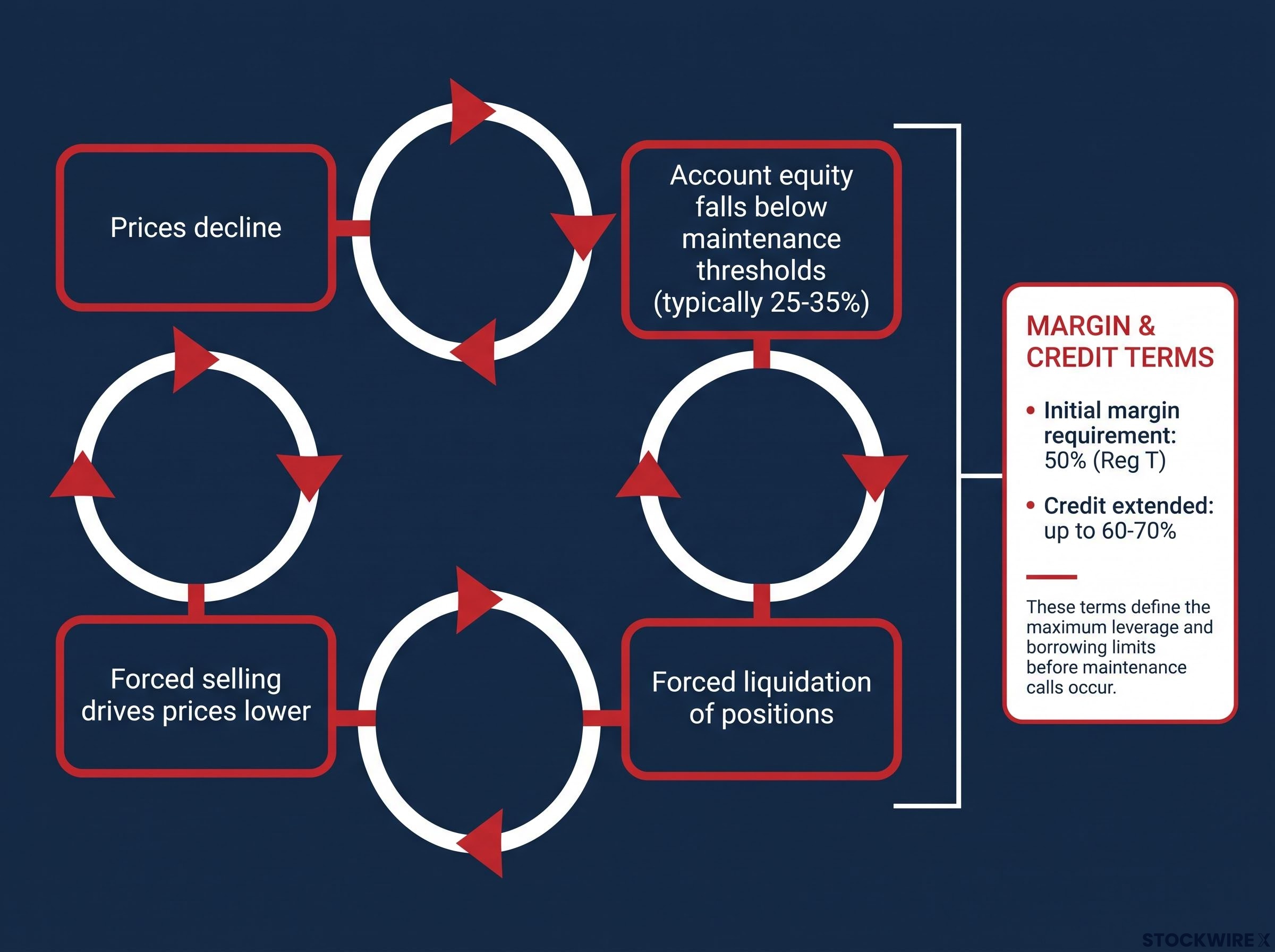
Under Regulation T (Reg T), the initial margin requirement for purchasing securities is 50%, meaning you must put up at least half the purchase price yourself. Lenders typically extend credit up to 60-70% of a borrower’s portfolio value, according to Clive Thompson, a veteran Swiss wealth manager and investment strategist. Beyond that point, the call comes.
“When borrowed capital amplifies gains on the way up, it works in reverse on the way down, with falling prices creating psychological and mechanical pressure to sell, each wave of selling pushing more accounts toward their limits and feeding the next round of forced liquidation.”
What matters for you, if you hold leveraged positions, is that the selling wave does not wait for a formal crash to be declared. Voluntary deleveraging begins well before maintenance thresholds are formally breached, as investors watching prices fall start selling to avoid the margin call they can see approaching. The forced selling that follows is the mechanism that pushes prices toward your limits next.
The difference in outcomes between being a forced seller (who must liquidate at dislocated prices) and a discretionary seller (who retains timing control) can be substantial.
Why semiconductors are the sector most exposed to a sentiment reversal
The semiconductor industry has a documented cyclical pattern that has repeated across memory chips, CPUs, smartphones, PCs, and crypto-related GPUs:
- Demand surges, creating supply shortages
- Capacity investment ramps to meet that demand
- Supply overshoots, producing excess inventory
- Chip prices compress, squeezing margins
- Earnings disappoint relative to elevated forecasts
This cycle is structural. It is not a feature of any single technology wave. It is a function of how capital-intensive manufacturing responds to demand signals with a time lag.
The AI demand cycle within a structurally cyclical industry
AI-driven demand has extended the current upcycle and created a temporary supply shortage that supports elevated chip prices and profit expectations. Clive Thompson’s analysis cites near-term semiconductor earnings growth estimates in the range of 30-50%, figures that have attracted significant buying activity.
The question for investors holding AI and semiconductor names is not whether the technology is real. It may well be transformational. The question is whether the earnings trajectory currently priced into valuations can survive the supply-demand normalisation that the industry’s own structure says is coming. Once capacity expands to meet and then exceed demand, the current earnings expectations embedded in prices become difficult to sustain.
The semiconductor cycle dynamics that make current earnings estimates structurally fragile are driven in part by TSMC’s locked-in 2026 capital budget of $52-56 billion and Samsung’s estimated $70-80 billion annual outlay, capacity commitments that make the 2027-2029 supply wave a structural certainty rather than a conditional risk.
Diversified revenue streams (automotive, industrial, networking) may moderate the correction for some firms, but they do not eliminate sector-wide valuation risk when consensus expectations reset.
The dot-com parallel applies directly here. The technology was real, the transformation was real, and investors who held at peak valuations still faced prolonged drawdowns. Being right on the technology does not protect against being wrong on the entry price.
What 1929, 1987, and 2000 actually teach about leverage and recovery
The instinct is to assume that a bigger crash means a longer recovery. The historical record complicates that assumption.
The single-day percentage decline in U.S. equities during the 1987 crash was approximately 22.6%, substantially larger than the 1929 single-day decline of approximately 13%. Yet 1987 produced no major recession. The underlying economy was sound, the liquidity response was aggressive, and markets recovered relatively rapidly.
1929, despite the smaller single-day fall, led to a prolonged economic depression that took decades for equity markets to recover from, because the banking system and broader economy were structurally fragile.
| Episode | Single-day decline | Recovery path | Primary lesson |
|---|---|---|---|
| 1929 | ~13% | Prolonged depression, decades to recover | Fragile economic conditions amplify aftermath |
| 1987 | ~22.6% | Rapid recovery, no major recession | Sound economy limits post-crash damage |
| 2000 | Gradual decline from March 2000 peak | Multi-year bear market | Correct valuation diagnosis does not confer timing precision |
The dot-com case introduces the timing problem most directly. Alan Greenspan delivered his “irrational exuberance” warning on 5 December 1996. He was analytically correct. He was also approximately three years early. Markets rose substantially before reaching their peak in March 2000.
The Greenspan episode shows how a correct analytical conclusion can still leave investors worse off if acted on too early. Those who cut exposure after his December 1996 speech sat out three years of substantial market gains before the correction they anticipated eventually materialised.
The meta-point: leverage amplifies whatever correction occurs, but the severity of the aftermath depends on economic context, not crash magnitude. That distinction matters more than the size of the initial decline.
NBER research on leverage and crises demonstrates that a stronger buildup of financial leverage during a boom phase tends to produce a deeper subsequent downturn, a finding that gives the current debt-to-cash ratio progression its historical weight.
The multiplicative effect when leverage and sector concentration overlap
Two risks tracked separately, record margin debt and semiconductor overvaluation, become a single compounding mechanism when you recognise they share the same collateral base.
The sector composition of margin collateral is not publicly disclosed. But the directional inference is structurally reasonable: AI and tech names dominate market capitalisation and have attracted the largest recent flows. A significant share of leveraged positions is almost certainly secured against these holdings.
Here is what that means. A valuation shock in semiconductor and AI equities would compress exactly the collateral backing the most leveraged positions, triggering margin calls in the names already under selling pressure. The forced liquidation would amplify the initial decline rather than dispersing it. Spill-over through ETFs and index futures would extend that pressure into broader indices.
The four conditions that produce this compounding effect:
- High leverage secured against high-beta, high-valuation assets
- Thin cash buffers (debt-to-cash ratio of approximately $6-$7:1)
- Sector concentration in assets facing potential earnings disappointment
- Non-discretionary forced selling as a mechanical amplifier
Research tracking margin debt cycles indicates that annual growth exceeding 40% has historically coincided with market peaks, with prior instances clustering around 2000, 2007, and 2021. Against those benchmarks, the current reading of 54% absolute margin debt growth and 26% excess growth stands above each of those prior thresholds.
This is the article’s central analytical claim: investors who have mentally accounted for semiconductor risk and margin debt risk as separate line items may still be underestimating their combined exposure, because the interaction is multiplicative, not additive. The feedback loop runs faster and deeper than either condition would produce in isolation.
Four questions investors should be asking their portfolios right now
The shift from “here is what is happening” to “here is how to think about where you stand” comes down to four diagnostic questions. These are not a checklist. They are stress-test lenses drawn from how institutional risk managers think about leveraged exposure.
- What is your direct and indirect leverage? Margin debt is the obvious form, but embedded leverage in options positions and leveraged ETFs can dramatically increase effective exposure without appearing on a margin statement.
- How concentrated are you in AI and semiconductor names? Over-concentration in the sectors that have led recent gains means your portfolio drawdown in a sentiment reversal could significantly exceed the index-level decline.
- What is your liquidity under stress conditions? Bid-ask spreads widen and market depth collapses in sharp corrections. Forced selling often occurs at dislocated prices, not at the last screen quote.
- Can your portfolio endure a sharper-than-expected drawdown without triggering a margin breach? The distinction between a forced seller and a discretionary holder is the most practically consequential variable you control.
Working through these questions honestly is not an exercise in predicting a crash. It is a stress-test of whether you retain the agency to act on your own terms if volatility arrives, rather than being forced to sell at the worst moment.
What a practitioner’s risk reduction actually looks like
Over the one to two months preceding mid-2026, Clive Thompson substantially trimmed his holdings in technology and semiconductor stocks while retaining a residual position rather than exiting the sectors entirely. This reflects an elevated risk assessment translated into portfolio posture under timing uncertainty, not a directional call or a recommendation.
It illustrates the practical response to the conditions described throughout this analysis: reducing concentration and reclaiming optionality while accepting that the correction, if it comes, may still be months or quarters away.
What changes if the correction arrives, and what does not
The conditions described here, record margin debt, semiconductor cycle risk, and multiplicative feedback potential, represent elevated risk architecture. They are not a crash prediction with a timeline.
Late-cycle positioning from major asset managers including BlackRock and J.P. Morgan has remained constructive through mid-2026, with both institutions characterising the Q1 sell-off as a cyclical correction rather than a structural reversal, a framing that sits in direct tension with the leverage architecture described here.
| What changes | What stays the same |
|---|---|
| The debt-to-cash ratio means a correction will likely move faster and further than it would in a lower-leverage environment | The distinction between being a forced seller and a discretionary holder remains the most controllable variable |
| Semiconductor earnings resets would compress the collateral backing leveraged positions, amplifying the drawdown | Sound underlying economic conditions can still limit post-correction damage (the 1987 lesson) |
| Spill-over through ETFs and index futures would spread sector-specific pressure into broader indices | Correct diagnosis of overvaluation does not confer timing precision (the Greenspan lesson) |
The practical response to elevated risk architecture is not to predict the correction. It is to audit your own position for forced-seller vulnerability, because that is the only variable you actually control. Investors who build their response around leverage, concentration, and liquidity buffers rather than around timing a market move are better positioned regardless of whether the anticipated correction arrives on schedule or continues to be delayed.
For readers wanting to translate the risk audit into a structural portfolio rebuild, our full explainer on post-60/40 portfolio construction covers how the stock-bond correlation has turned positive during inflation shocks and what a three-tier adaptive framework looks like in practice.
This article is for informational purposes only and should not be considered financial advice. Investors should conduct their own research and consult with financial professionals before making investment decisions. Past performance does not guarantee future results. Financial projections are subject to market conditions and various risk factors.