Most investors think about their holdings in simple terms: you own a stock, the price goes up, and your portfolio is worth more. End of story. In a leveraged financial system, that is only the first move in a much longer sequence.
Here is the scale that makes it matter. With an estimated $30 trillion in global leveraged equity exposure, according to Cem Karsan of Kai Volatility Advisors, a 10% market gain generates roughly $3 trillion in fresh collateral available for recycling within days. That is new purchasing power created almost automatically, and it does not sit idle.
This dynamic clusters in the 48-hour window around month-end and quarter-end, and it is a structural feature of the system rather than a calendar quirk. The context is substantial: global equity market capitalisation reached approximately $155-158 trillion in 2025 (SIFMA and WFE), and U.S. margin debt hit a record $1.50 trillion in June 2026 before settling at $1.45 trillion in August 2026, up 37% year-on-year (FINRA).
After reading this, you will understand why sophisticated participants treat quarter-end windows as structural opportunities, and what conditions determine whether those windows actually deliver.
What actually happens when markets rise: the collateral recycling loop
Start with the mental model you probably hold. Prices rise, your position gains value, and that is the whole event. In a system where most capital is borrowed against, the gain is not a terminal event. It is a trigger.
The majority of global capital is deployed with leverage, through credit, loans, margin accounts, and structured instruments. When asset prices rise, the value of the collateral backing those borrowings rises too. That expands how much can be borrowed, which funds new positions, which supports prices further.
The sequence runs like this:
- Prices rise across leveraged positions.
- The collateral base supporting those positions expands in value.
- Borrowing capacity increases, because lenders will advance more against higher-valued collateral.
- New positions are opened using that expanded capacity, feeding back into prices.

The collateral maths With roughly $30 trillion in estimated global leveraged equity exposure, a 10% market gain creates approximately $3 trillion in new collateral available for releveraging. That capital does not wait. It re-enters the market.
What makes this loop structural rather than discretionary is that it is not a choice anyone sits down to make. It follows from rule-based risk systems, margin agreements, and secured-funding haircut schedules that automatically adjust the moment asset values move.
From individual margin accounts to system-wide procyclicality
The same mechanism that operates on a single margin account scales to the entire financial system. On your account, asset value up means available credit up. Across the system, the same logic runs through repo haircuts, derivatives collateral, and bank capital ratios.
Research by Tobias Adrian and Hyun Song Shin shows that financial intermediaries manage their balance sheets to target a Value-at-Risk or leverage ratio, a measure of how much they could lose or how much they have borrowed relative to capital. When prices rise and volatility falls, measured risk drops, so those institutions mechanically expand their balance sheets and buy more.
BIS and central-bank studies on margining confirm the amplifier. In benign periods, haircuts on secured financing fall, which frees additional collateral capacity across the whole system at once.
Repo market haircuts are one of the most direct transmission channels through which a shift in funding conditions reaches leveraged equity portfolios; when haircuts on secured financing rise, the same collateral base that expanded borrowing capacity in benign conditions suddenly supports less, compressing balance sheets across the system simultaneously.
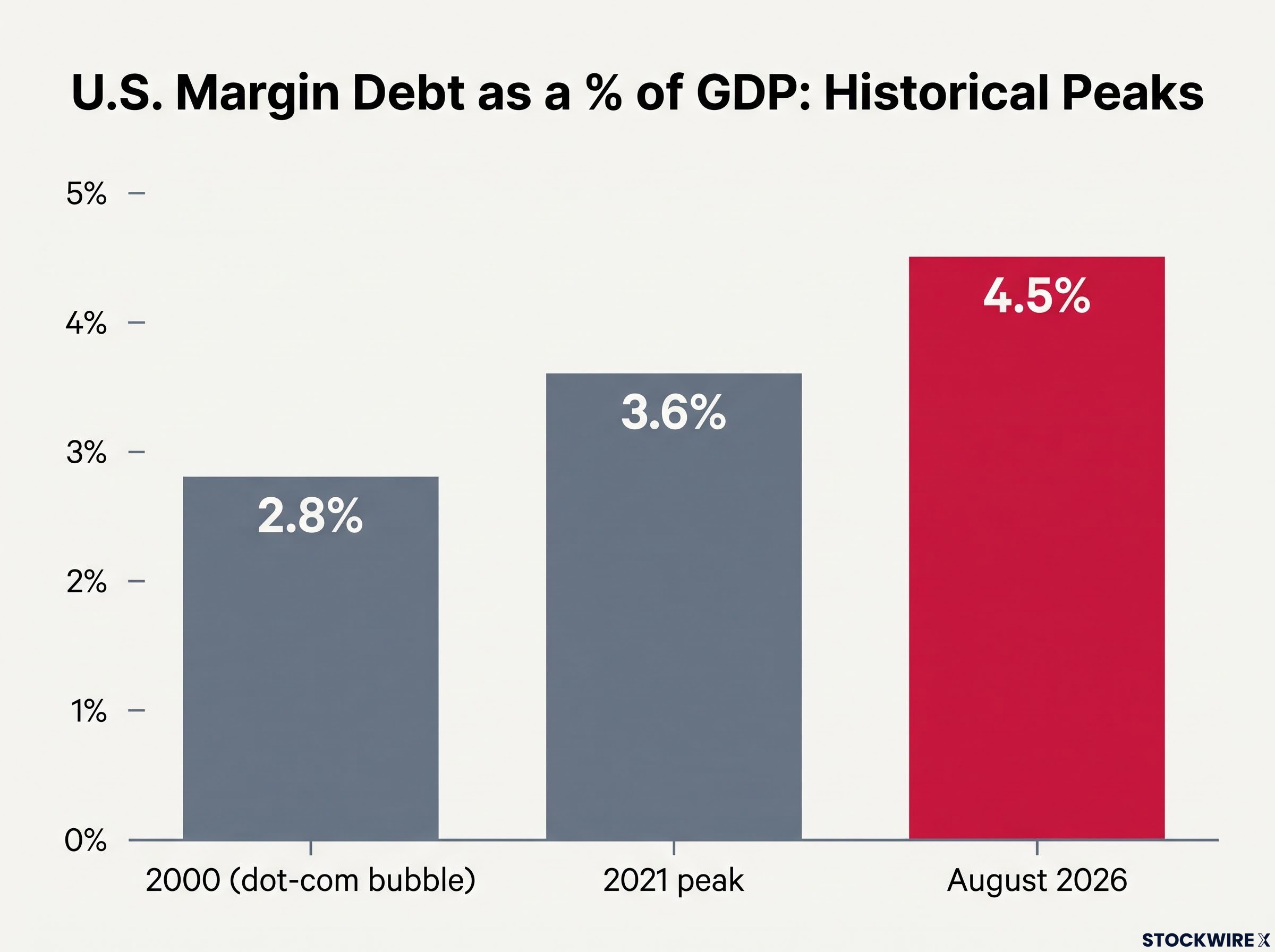
Here is what the scale tells you. U.S. margin debt now sits at approximately 4.5% of U.S. GDP, above the 3.6% peak in 2021 and well above the 2.8% level near the 2000 dot-com bubble. The collateral recycling engine is running at historically elevated intensity, which amplifies both the quarter-end tailwinds in good conditions and the severity of the reverse loop if conditions turn.
When big ASX news breaks, our subscribers know first
Why quarter-end intensifies the loop: accounting marks and institutional incentives
The mechanics explain why rising prices create new buying. They do not yet explain why that buying concentrates at the end of a quarter. The answer shifts from the mechanical to the institutional.
Quarter-end accounting marks set the leverage ratios that banks and corporations rely on for their borrowing and lending capacity throughout the following quarter. A higher quarter-end print is not a one-day cosmetic win. It supports greater balance-sheet activity for months.
That gives several groups of actors concentrated reasons to want prices high at the exact moment the snapshot is taken:
- Banks and dealers: leverage ratios, liquidity coverage ratios, and capital requirements are calculated at reporting dates, creating incentive to optimise the balance sheet cosmetically.
- Pension and insurance funds: strategic weights and funding ratios are assessed against period-end valuations.
- Hedge funds: reporting marks influence prime-brokerage terms and investor-facing performance.
- Corporate treasury: collateral values at the mark determine subsequent borrowing capacity.
This is the window-dressing dynamic. Institutions temporarily adjust repo books, derivatives inventories, and securities holdings before the reporting snapshot, then re-expand positions once the mark is recorded.
Karsan has pointed to late March as an illustration, when a run of policy-related announcements coincided with a strong rally into quarter-close, with the market-moving items appearing to concentrate around the 29th and 30th. In the Q3 context he discussed, with the S&P 500 up roughly 3% for the quarter, the structural rebalancing environment was net positive.
The read you should take is this. The final two trading days of a quarter are not neutral ground. Actors with explicit regulatory obligations have structural reasons to support prices right then, so treat the window as a convergence of mechanical and administrative forces, not a single clean flow.
The hierarchy of calendar transitions
Not every calendar boundary carries the same weight. There is a clear ranking.
| Transition type | Frequency | Primary driver | Historical analogue |
|---|---|---|---|
| Month-end | Monthly | Simple monthly mark and rebalancing | Routine month-end flows |
| Quarter-end | Quarterly | Leverage and capital ratio reporting marks | Amplified month-end effect |
| Year-end | Annually | Longest collateral build plus highest-stakes mark | Santa Claus rally, January effect |
Year-end is the strongest because it combines the longest collateral accumulation period with the most consequential reporting mark. Quarter-end amplifies the month-end effect because leverage and capital ratios matter more than a routine monthly mark. Sophisticated participants treat this hierarchy as a scaling factor when sizing positions ahead of each transition.
Front-running the structural flow: how sophisticated participants position ahead of quarter-end
If the timing and direction of a flow are broadly understood, that knowledge becomes a positioning problem. Everyone who sees it coming wants to be in before it arrives.
The timing and direction of quarter-end releveraging flows are widely understood among institutional participants. That creates a direct incentive to enter positions days before the window, in anticipation of the structural buying that the collateral loop and accounting marks will produce.
The result is that the flow front-runs itself. The layers typically enter in this order:
- The earliest discretionary movers, who position days ahead based on flow estimates.
- Systematic strategies, including volatility-targeting funds and risk-parity portfolios, that mechanically raise equity allocation as volatility stays suppressed and prices rise.
- The structural flow itself: the mechanical collateral recycling and accounting-mark buying over the final sessions.
The structural window, defined Karsan frames the core opportunity as the 48-hour period spanning the final day of a month and the first day of the next, with quarter transitions amplifying the effect.
This anticipation compresses the window. The bulk of the move can occur before the final day of the month, as successive layers try to get ahead of each other. By the time the last trading day arrives, much of the structural bid may already be in the price.
That matters for how you read the window. The actionable edge sits earlier than it appears, and it lies in understanding the flow mechanics well enough to position ahead of the crowd that is already positioning ahead. The informational asymmetry is real, because most retail participants think in unlevered terms and miss the mechanism entirely.
The options market overlay
There is a derivatives layer sitting on top of the equity flow. Dealer gamma and vega exposure around options expiries and month-end can either dampen or amplify equity moves, depending on whether market makers are net long or short gamma at the time.
Dealer gamma positioning around options expiries operates as a structural layer on top of the equity flow mechanics, with net short gamma regimes causing market makers to extend rather than cushion directional moves, a dynamic that can either amplify or compete with the quarter-end releveraging bid depending on the calendar overlap.
Institutional option rolls and structured-product resets tend to cluster near calendar boundaries. In favourable conditions, that adds a derivatives-driven bid to the underlying structural flow, compounding the directional bias. It is a supporting mechanism, not the core of the story.
When the window fails: conditions that override the structural bid
“It does not always work” is useless as guidance. What you need is a way to tell a favourable setup from an unfavourable one before the window opens.
The effect is state-dependent. The sign and magnitude of flows are determined by prior performance, volatility conditions, and funding stress, and all three can turn the structural bid into structural selling.
| Condition | Favourable setup | Unfavourable setup |
|---|---|---|
| Prior quarter equity performance | Solid gains that expand collateral | Strong equity outperformance forcing rebalancing sales |
| Volatility environment | Suppressed realised and implied volatility | Volatility spike raising measured risk |
| Funding and haircut conditions | Easy funding, low haircuts | Rising haircuts and margin calls |
| Institutional rebalancing obligations | No dominant obligation to sell equities | Mandated equity selling to restore weights |
The rebalancing reversal is the most common trap. If equities have strongly outperformed bonds during the quarter, large pension and endowment allocators may be required to sell equities and buy the underperforming assets to restore strategic weights. That net selling can compete with or overwhelm the releveraging bid.
Institutional rebalancing flows at quarter-end are not always directionally positive for equities; when bonds have sharply underperformed, the world’s largest pension allocators face mandatory obligations to sell equities and buy fixed income that can overwhelm the releveraging bid described above.
The crisis override is the more severe one. In high-volatility or funding-stress regimes, rising haircuts and margin calls force deleveraging regardless of reporting incentives, turning the same collateral-sensitivity mechanism into a source of selling.
Front-running itself fails in four specific ways:
- The sign of the flow is misjudged, because asset-class performance or volatility evolved differently than the models expected.
- A policy announcement or data surprise lands near quarter-end and overshadows the structural flow.
- Institutions shift to continuous or algorithmic rebalancing, smearing flows over time rather than concentrating them in 48 hours.
- A crisis regime forces deleveraging that overwhelms any reporting-date incentive.
Here is the uncomfortable symmetry. The conditions that make the window work, prior gains, low volatility, easy funding, are the same conditions that make its failure mode most violent. The leverage that powers the structural bid becomes the mechanism of the structural unwind if any enabling condition breaks near the mark.
The systemic amplifier hiding in plain sight
The elevated level of U.S. margin debt is not just a backdrop figure. It calibrates how much is at stake.
At approximately 4.5% of GDP in August 2026, margin debt sits above the 3.6% peak of 2021 and the 2.8% level near the 2000 dot-com bubble. That means the procyclical leverage mechanism is operating at greater scale than in prior cycles, amplifying both the quarter-end tailwinds in good conditions and the speed of the reverse loop in bad ones.
The same debt-to-cash compression that powers the collateral recycling loop in benign conditions creates a forced-selling feedback loop in stress: when margin borrowers collectively owe more than they hold in available cash, a price decline triggers margin calls in the names already under selling pressure, multiplying rather than adding to the initial shock.
One further layer deserves a flag. Hedge fund gross borrowing was estimated at roughly $7.2 trillion with gross leverage near 10x (an unverified Seeking Alpha estimate cited via TheStreet, July 2026). If accurate, that adds another dimension of system-wide leverage sensitivity to the collateral dynamics described throughout. Treat the figure as indicative rather than confirmed.
Reading the quarter-end setup before the window opens
You do not need a trading rule. You need a filter: a way to tell, before the window opens, whether the structural forces are likely to be working with you or absent and reversed.
Run the setup against four prerequisites for a structurally favourable window:
- Positive prior-quarter equity performance that has expanded the collateral base.
- Suppressed realised and implied volatility.
- Easy secured-funding conditions with low haircuts.
- No dominant institutional obligation to sell equities for rebalancing.
The core principle The majority of global capital is deployed with leverage, so market gains automatically generate new collateral that recycles back into the market. That is the engine behind the entire quarter-end effect.
The 2025-2026 environment, with global equity market capitalisation up approximately 18-19% to around $155-158 trillion and U.S. margin debt up 37% year-on-year, is a period when this engine has been running at high intensity. That makes structural flow awareness especially relevant now.
Keep the hierarchy in mind as a magnitude guide: year-end transitions are historically the most powerful, quarter-end the second, month-end the third.
Treat Karsan’s framework as a lens, not a signal. It explains why certain windows tend to attract institutional support. It does not predict exact magnitudes or remove execution risk. Most retail participants miss all of this because they analyse markets in unlevered terms, treating each period as a blank slate. You now have visibility into a persistent structural feature of the system that institutions actively use to frame their positioning.
This article is for informational purposes only and should not be considered financial advice. Investors should conduct their own research and consult with financial professionals before making investment decisions. Past performance does not guarantee future results, and these structural flow dynamics are state-dependent and subject to change based on market conditions.