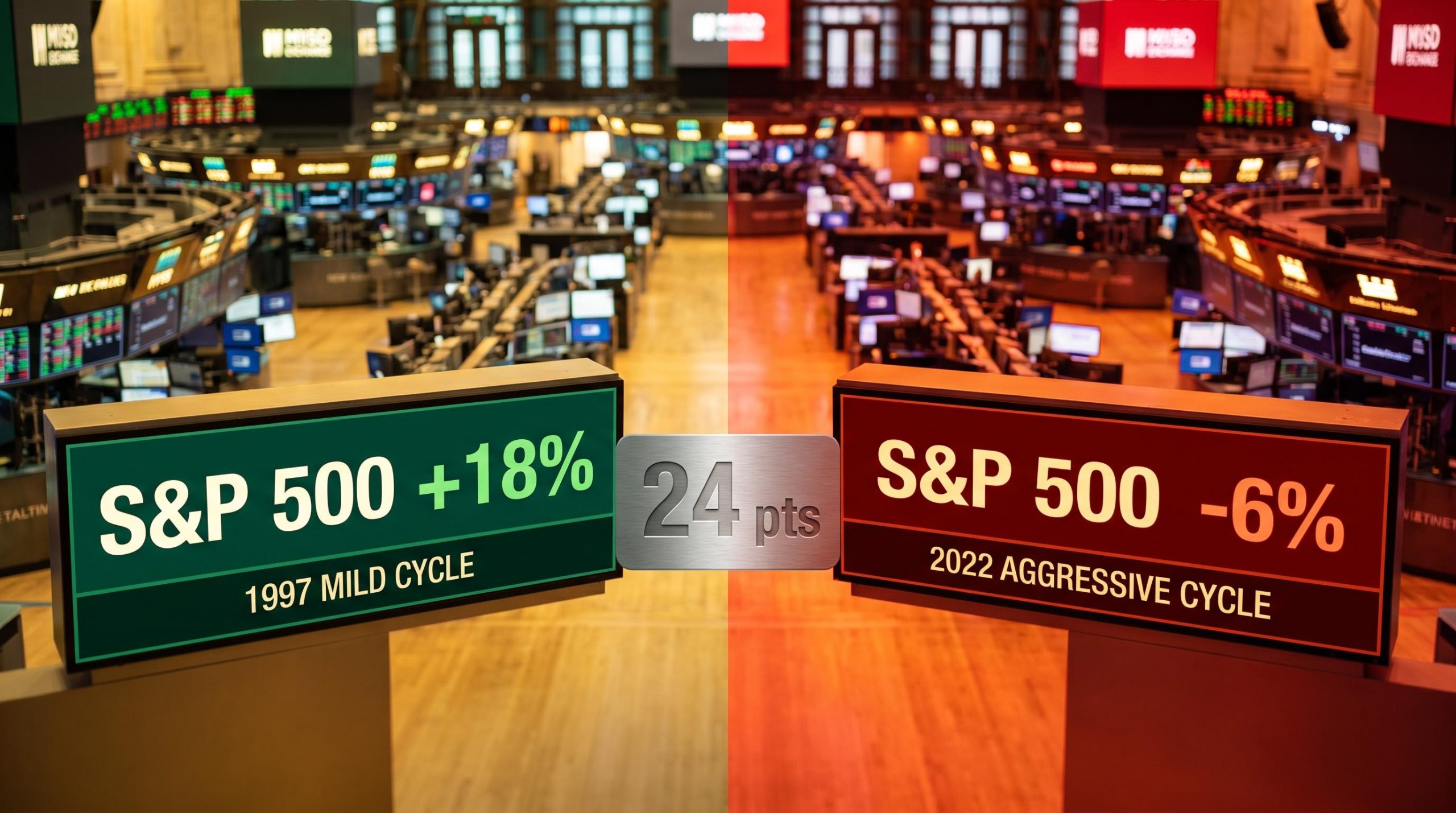
Two Federal Reserve tightening cycles can each lift interest rates by 300 basis points and hand you completely opposite outcomes. In March 1997, the Fed delivered a single hike, and the S&P 500 climbed 18% over the following four months. In 2022, the Fed delivered eleven hikes in a compressed campaign, and the index fell roughly 6% over the same window.
Same direction. Rates went up in both. The results were nearly a quarter of the index apart.
That contrast matters right now because the Fed is not moving. It has held the federal funds rate at 3.50-3.75% since the beginning of 2026, and the direction of the next major move is genuinely uncertain. Whether that next cycle turns out mild or aggressive will shape portfolio positioning far more than most investors expect.
Here is what the historical record actually tells you: how to read the character of a tightening cycle, not just its direction. Get that read right at the outset, and you have a clearer view of which sectors will carry a portfolio through it, well before the market finishes pricing the answer.
The 24-point gap: what mild and aggressive cycles have actually done to the S&P 500
Start with the gentlest cycle on record and work upward. The pattern is easier to see when the numbers arrive in order of severity rather than all at once.
According to analysis presented by Tapper Strickland, chief market strategist for Mumu, the single hike of March 1997 was followed by an 18% gain in the S&P 500 over four months. The 1999 cycle, another mild campaign, produced a rise of roughly 4% across the same window. The 2004 cycle delivered a gain of about 6%.
Then the character shifts. The 1994 aggressive cycle saw the index fall approximately 6% over four months. The 2022 aggressive cycle, eleven hikes taking rates from near zero toward a peak of 5.25-5.50%, produced a decline of roughly 6% as well.
Goldman Sachs data on S&P 500 performance during rate hikes shows the index averaging roughly 9% in the 12 months following the first hike of a cycle, with the 2022 episode identified as an outlier driven by emergency-pace tightening and elevated starting valuations rather than a template for how most campaigns unfold.
| Cycle Year | Cycle Type | Number of Hikes | Increment Size | S&P 500 Return (4 months) |
|---|---|---|---|---|
| 1997 | Mild | Single hike | 25 bps | +18% |
| 2004 | Mild | Limited | 25 bps | +6% |
| 1999 | Mild | Limited | 25 bps | +4% |
| 1994 | Aggressive | Frequent | Above 25 bps | -6% |
| 2022 | Aggressive | 11 hikes | Above 25 bps | -6% |
The definitions are worth fixing in place. A mild cycle involves 25-basis-point increments and a limited number of hikes. An aggressive cycle involves larger increments delivered more frequently over a compressed period.
The spread that matters: +3% to +18% in mild cycles versus approximately -6% in aggressive cycles over the same four-month window.
Why four months captures the character effect
That gap between the best mild outcome and the worst aggressive one runs to roughly 24 percentage points. It is not noise, and it points to something practical: classifying the cycle correctly at its start is a more actionable skill than forecasting where rates finally settle.
Four months is the window because it isolates the market’s reaction to the cycle’s character before the slower-moving data arrives. In that period, GDP figures and corporate earnings have not yet shifted meaningfully in response to the new rate path.
Push the measurement window out further and the pure rate-path signal gets buried. Beyond four months, macro outcomes and earnings revisions start to dominate, and you are no longer measuring the market’s read on the cycle’s character. You are measuring the economy that character produced.
When big ASX news breaks, our subscribers know first
Three transmission channels that explain why pace matters more than destination
Why does pace beat destination? Because the damage from aggressive tightening travels through a chain, and each link makes the next one worse. Understanding that chain is what turns pattern recognition into a live analytical toolkit.
The first link is the discount rate. When rates rise quickly, the rate used to value future company cash flows rises with them, and price-to-earnings multiples compress. Research by Bernanke and Kuttner (American Economic Review, 2005) found that unexpected rate hikes push equity prices down through both higher discount rates and a higher equity risk premium, the extra return investors demand for holding stocks over risk-free bonds.
The three channels work in sequence, not in parallel:
- Discount rate compression: Under mild conditions, telegraphed hikes let the equity risk premium adjust gradually. Under aggressive conditions, the entire expected policy path jumps at once, hammering long-duration growth assets whose value sits in distant future earnings.
- Earnings forecast revisions: Under mild conditions, analysts trim estimates slowly as growth softens. Under aggressive conditions, rising recession risk triggers sharp forecast cuts in cyclical sectors including industrials, consumer discretionary, and smaller caps.
- Credit condition tightening: Under mild conditions, loan growth slows but funding stays available. Under aggressive conditions, spreads widen and lending standards tighten, choking off refinancing for indebted firms.
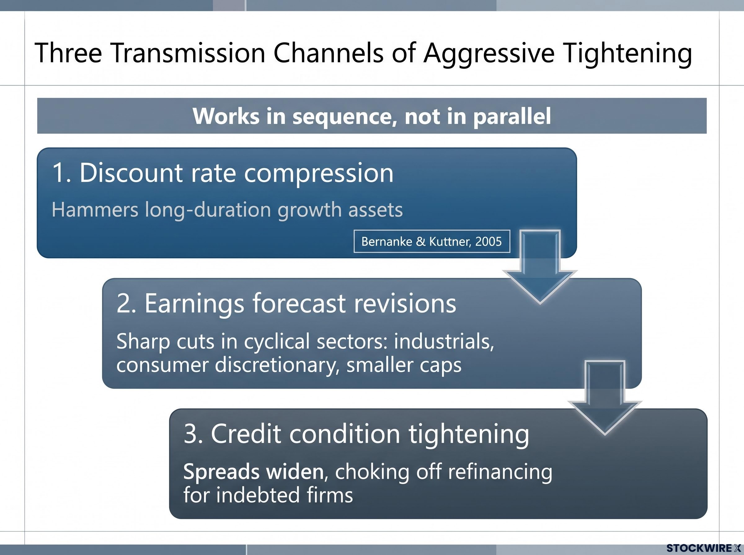
Notice what the chain does. Aggressive cycles do not simply lower stock prices through a one-off multiple contraction. They degrade the quality of the earnings environment those prices rest on, which is why recovering from an aggressive cycle takes longer than a straightforward re-rating once rates stabilise.
Credit stress as the amplifier
The credit channel is the one that compounds the other two. When spreads widen and lending standards tighten, the pain concentrates in high-yield issuers and leveraged-loan borrowers who suddenly find refinancing expensive or unavailable.
Research from the BIS and IMF stresses that aggressive tightening interacts with high leverage and maturity mismatches to produce outsized stress, even when headline macro data still looks resilient. That gap between resilient headlines and building stress is exactly where investors get caught.
The 2023 regional bank episode was a live illustration. Rapid hikes produced large unrealised losses on long-duration securities portfolios, while an inverted yield curve compressed net interest margins, overwhelming the rate benefit that financials are traditionally assumed to capture. For monitoring purposes, this tells you to watch credit spreads, forward earnings revisions, and the shape of the yield curve, not just the rate announcements themselves.
Sector rotation playbook across cycle types
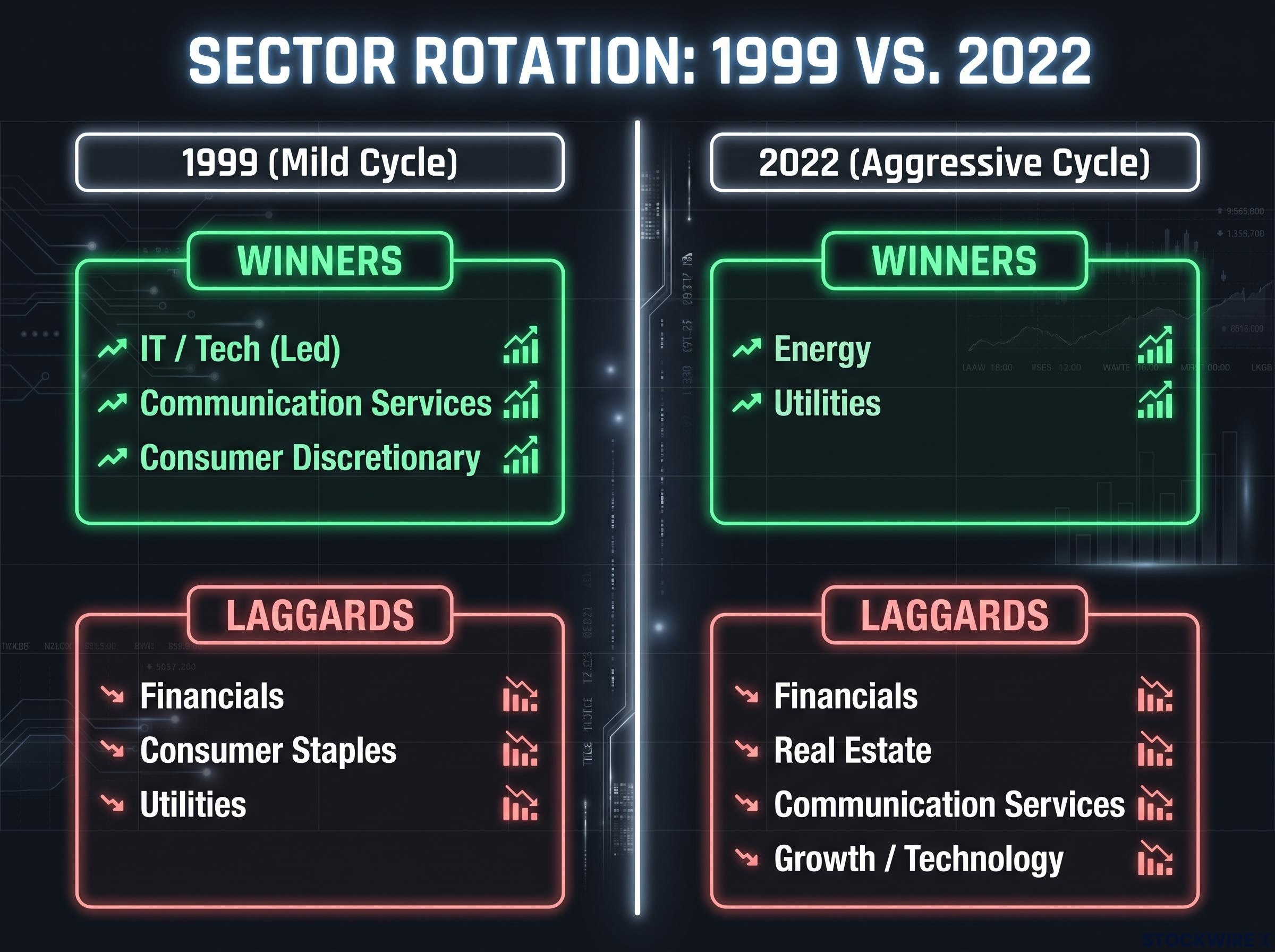
The clearest way to see sector behaviour is to put two cycles side by side. In 1999, a mild cycle, the IT sector led the market over the four months following the first hike. Communication services and consumer discretionary outperformed, while financials, consumer staples, and utilities lagged.
In 2022, an aggressive cycle, the map inverted. Energy and utilities gained, while financials, real estate, and communication services underperformed, and growth and technology names took large drawdowns.
| Sector | Mild Cycle Tendency | Aggressive Cycle Tendency | Key Driver |
|---|---|---|---|
| Technology / Growth | Leads | Large drawdowns | Discount rate sensitivity |
| Consumer Discretionary | Outperforms | Pressured | Recession risk, sentiment |
| Financials (Banks) | Mixed | Underperforms if curve inverts | Net interest margin, curve shape |
| Financials (Insurance) | Benefits | Benefits | Higher portfolio income |
| Real Estate / REITs | Lags | Underperforms | Higher cap rates, mortgage rates |
| Energy | Neutral | Gains on supply shocks | Inflation composition |
| Consumer Staples / Utilities | Lags | Defensive gains | Recession hedging |
Here is where the simple version breaks down. Post-2022 commentary from Goldman Sachs and Morgan Stanley has argued that “technology outperforms in mild cycles” is too crude a rule. What actually determines outcomes is the combination of starting valuations, real-rate moves, and earnings resilience.
The 2022 rotation looked different from a purely growth-driven aggressive cycle because its inflation was energy and goods driven, which lifted energy producer cash flows even as discount rates crushed long-duration names. The insurance industry offers another wrinkle: unlike banks, insurers tend to benefit from rising rates through higher income on the fixed-income holdings that match their liabilities.
The read for you is that the sector map is regime-dependent, not a fixed set of rules. Diagnose the interaction of rate pace, curve shape, inflation source, and starting valuation. Do not simply identify which way rates are heading.
Why the bank outperformance thesis needs a yield curve qualifier
The idea that banks win during rate hikes rests on one assumption: a normally shaped yield curve. Banks make money on the gap between what they pay depositors short term and what they earn on lending long term.
Yield curve shape is the single most important qualifier on the bank thesis: a steepening curve loosens credit supply by improving net interest margins and making new loan origination more economically attractive, while a compressing or inverted curve does the opposite, turning the theoretical rate tailwind into a funding and earnings headwind of the kind that produced the 2023 regional bank stress.
Invert that curve and the logic reverses. Short-term deposit costs rise faster than long-term lending yields, compressing net interest margins rather than expanding them.
The 2023 regional bank stress showed this playing out. Aggressive tightening turned a theoretical rate tailwind into an actual funding and earnings headwind, with deposit flight and unrealised securities losses stacking on top. Before assuming financials are a rate-hike winner, check the curve.
What the historical record cannot tell you: the limits of cycle analogies
None of this makes the framework a set of forecasts. The caveats below are not disclaimers that weaken the analysis; they are the layer that separates an investor who applies the framework with judgment from one who matches cycle labels mechanically.
Three structural differences limit direct historical comparison. Treat each as a diagnostic question to ask when a new cycle emerges:
- What are the starting valuations and macro regime? When equities begin rich, even a mild cycle can trigger a meaningful de-rating. Post-pandemic conditions featured unusually high inflation and distorted household savings, unlike 1994 or 2004.
- How are balance sheets composed? Large corporates now carry higher fixed-rate debt shares and larger cash cushions, reducing their direct sensitivity to short-rate moves. Smaller, bank-dependent, and highly leveraged firms remain far more exposed.
- Is quantitative tightening in play? Recent cycles pair rate hikes with balance-sheet reduction, altering term premia and global dollar liquidity in ways earlier episodes never captured.
There is a fourth diagnostic that sits above the rest: the source of the inflation. The 2022 cycle was driven by an energy and goods shock rather than demand overheating, and that alone reshaped its sector rotation compared with growth-driven aggressive cycles. Identify the inflation source first.
Inflation composition is the variable the standard cycle-classification framework handles least cleanly: August 2026 headline CPI rose to 3.4% on energy and telecoms supply shocks while core held at 2.4% and continued decelerating, a split that matters because rate tools have no direct transmission mechanism to supply-driven price pressure, making the policy calculus different from demand-overheating episodes like 1994.
The Fed’s own caution: Recent Monetary Policy Reports have repeatedly warned that uncertainty around the neutral rate and inflation dynamics reduces the reliability of past cycles as guides.
The BIS and OECD add that passive investing, algorithmic trading, and integrated global capital markets amplify reactions to policy surprises, making modern cycles more prone to sharp cross-asset moves. What this means for you is straightforward: use the historical data to form a hypothesis about regime type, then stress-test that hypothesis against current balance-sheet and inflation conditions rather than trusting the label alone.
Reading the character of the current cycle before it moves
So how do you apply this while the Fed sits still? The baseline as of the July 2026 FOMC statement is a hold at 3.50-3.75%, with no active tightening or easing. The useful question is not which way the Fed moves next. It is: if a new tightening cycle begins, what early signals will let you classify its character before the damage is done?
The three transmission channels convert neatly into three observable signals:
- Credit spread behaviour: Widening spreads early in a cycle point toward aggressive conditions and flag risk for high-yield issuers and leveraged borrowers first.
- Yield curve shape: A normal curve supports the traditional bank thesis; an inverted curve reverses it and signals margin pressure across financials.
- Forward earnings revisions in cyclicals: Sharp downward revisions in industrials, consumer discretionary, and smaller caps indicate the market is pricing recession risk, a hallmark of aggressive cycles.
The starting point itself is a signal. Current rates already reflect an aggressive prior cycle, so any new campaign would begin from a materially different place than 2022’s near-zero origin.
Sector positioning before the cycle declares itself
If early signals lean mild, the historical winners come back into focus. Technology and consumer discretionary led in 1999, and consumer discretionary was trading roughly 30% below its 52-week highs at the time of the referenced broadcast, which suggests negative sentiment may already be priced in should a mild cycle materialise.
If signals lean aggressive, the defensive tilt has historical support. Lean away from rate-sensitive REITs and leveraged small caps, particularly with the 30-year fixed mortgage rate at 6.71% as of 3 September 2026, a structural drag on real estate and homebuilders regardless of cycle character.
One caution against mechanical application: even in the aggressive 2022 cycle, mega-cap technology leaders with strong balance sheets and secular earnings drivers recovered sharply in 2023, faster than the cycle-character framework alone would predict.
Classifying the cycle is the analysis, not the output
Return to the two bookends. In 1997, one hike and the S&P 500 up 18% over four months. In 2022, eleven hikes and the index down 6% over the same window. The direction was identical; the character produced a spread of roughly 24 percentage points.
That is the whole point. The direction of rate moves matters less than their character, meaning the pace, the increment size, the inflation regime, and the curve shape. History hands you a template for diagnosing that character before markets have finished pricing what it implies.
Meeting-by-meeting rate predictions have become structurally less reliable under Kevin Warsh’s guidance-free communication framework, which is designed to keep policy options open at every FOMC meeting, meaning the cycle-character approach described here is not just a complement to rate-direction forecasting but a partial replacement for it in the current regime.
Keep this in view: the roughly 24-percentage-point spread between the best mild-cycle outcome and the worst aggressive-cycle outcome is why classifying the cycle is a high-value analytical input, not an afterthought.
The current hold at 3.50-3.75%, sustained through 2026, is not a dead zone. It is the window in which the diagnostic signals are forming, which makes it the ideal time to build the framework rather than scramble once a cycle is already underway. Investors who approach the next cycle asking “what kind of cycle is this?” rather than “which way are rates going?” are positioned to see it coming instead of reacting after the fact.
This article is for informational purposes only and should not be considered financial advice. Investors should conduct their own research and consult with financial professionals before making investment decisions. Past performance does not guarantee future results. Financial projections are subject to market conditions and various risk factors.