
The same administration that is raising the ceiling on long-end Treasury buybacks to suppress borrowing costs announced what it calls the most sweeping financial measures ever directed at Iran, all within the same news cycle. One tool is designed to put downward pressure on long-term yields. The other risks pushing them sharply higher through an oil-driven inflation channel.
On 24 August 2026, these two developments collided. The long-end buyback ceiling was raised to a minimum of $4 billion per operation, effective 9 September, and the Iran sanctions announcement was scheduled for 18:00 GMT the same day. Neither development can be assessed in isolation. The buyback programme is a technical bid for the long end; the sanctions threaten to inject an inflation risk premium that overwhelms it.
The practical question this analysis resolves: which force is likely to dominate over the 9 September to 4 November window, and what should a bond or energy investor monitor to know how the balance is shifting in real time.
How the Treasury’s expanded buyback programme actually works
The Treasury announced the new operational parameters on 19 August 2026. The mechanics are straightforward, but the market interpretation layered on top of them is where confusion begins.
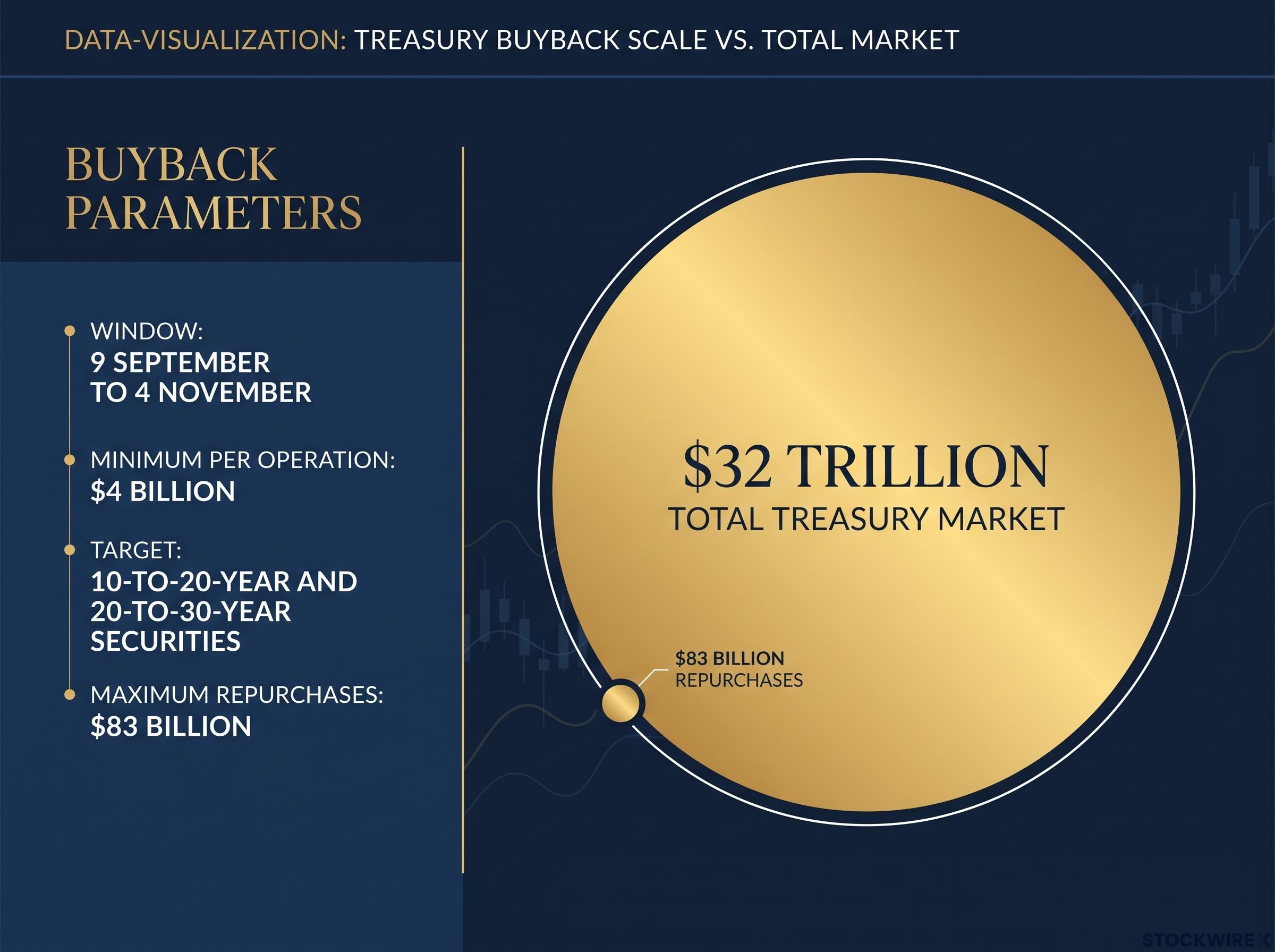
Here are the four operational parameters:
- Ceiling size: Minimum $4 billion per operation, doubled from the prior $2 billion limit
- Securities covered: 10-to-20-year and 20-to-30-year nominal coupon securities
- Effective dates: 9 September through 4 November
- Financing mechanism: Proceeds from new obligations and general funds, per Treasury’s statutory authority
The programme’s stated purpose is liquidity support for off-the-run issues, the older, less-liquid bonds that trade at wider spreads than their on-the-run equivalents. That is not yield-curve control. It is not a formal commitment to suppress long-term rates. The distinction matters because it determines how much weight markets can place on the programme if conditions deteriorate.
Maximum long-end repurchases for the window are estimated at approximately $83 billion, adding roughly $14 billion of extra capacity. Set that against the total Treasury market of approximately $32 trillion. The operations work through signal and predictability, not raw volume, which means the programme’s effectiveness depends heavily on whether markets trust the commitment.
Why the “twist” label is analytically useful but misleading as policy description
The Treasury Secretary applied the “twist” label to the buyback programme. That characterisation conveys the underlying logic: retiring longer-dated securities while selling shorter-term paper compresses average maturity without shrinking the total stock of government obligations. It is, however, an interpretive gloss applied from outside, not the language Treasury itself used to frame the initiative.
The “twist” framing is analytically useful for understanding the economic effect, but it is not a stated policy objective. Treasury’s official language emphasises market functioning and liquidity support, not yield-curve management.
The twist effect is only real if new issuance simultaneously tilts toward shorter maturities. You cannot read the net duration impact from the buybacks alone. And shortening average maturity carries a concrete cost: a greater share of the federal government’s interest burden becomes sensitive to wherever the policy rate sits at any given moment. Federal interest expenditure has already crossed $1.1 trillion for the current fiscal year, so the sensitivity of that bill to short-term rates is a live fiscal concern, not a theoretical one.
The Operation Twist precedent is the most instructive historical benchmark here: the 2011-2012 Maturity Extension Programme, operating under far more favourable conditions, delivered only around 15 basis points of long-end yield reduction, which sets a practical ceiling on what the current bounded programme can achieve through the signalling channel alone.
When big ASX news breaks, our subscribers know first
The $950 billion TGA and what it means for banking system liquidity
The Treasury General Account (TGA) functions as the federal government’s primary cash account held at the Federal Reserve. Think of it as the Treasury’s cheque book. When it rises, money leaves the banking system. When it falls, money flows back in.
As of the current period, the TGA stands at close to $950 billion, which is roughly $350 billion higher than the operational level at which the previous administration typically ran the account. That gap represents a genuine liquidity overhang.
Here is the mechanism. When Treasury draws down the TGA to fund spending or buybacks, those funds flow into bank accounts held at the Fed. Reserves in the banking system rise mechanically, independent of any Fed action. Officials have stated they expect funds exiting the TGA to flow into banking system reserves. This is shadow easing: a liquidity injection that looks nothing like a rate cut but functions as one in money markets.
The fiscal-side transmission from the TGA into banking reserves is already visible in dollar markets: the Dollar Index broke below its 200-day EMA even as long-end yields fell, a cross-asset pattern consistent with reserve injection rather than Fed easing.
| TGA scenario | Reserve flow | Liquidity effect | Key dependency |
|---|---|---|---|
| High TGA maintained | Reserves withdrawn | Tightening | Depends on bill issuance pace |
| TGA drawdown to fund spending | Reserves injected | Easing | Depends on offset from new bill issuance |
| TGA drawdown partially offset by bill issuance | Reserves partially injected | Neutral to mild easing | Depends on issuance volume |
Two caveats keep the story honest:
- Bill issuance offset: If long-end buybacks are financed by additional bill issuance rather than a pure TGA drawdown, the reserve injection is partially offset by cash raised from markets, weakening the shadow-easing narrative
- Fed facility interactions: The degree to which reserve additions ease overnight rates depends on the configuration of the Fed’s standing facilities and any remaining overnight reverse repo usage
Most bond market commentary focuses exclusively on the Fed. The TGA is a second, underappreciated liquidity variable that can move markets independently. If you track it alongside the Fed’s balance sheet, you gain a view of the plumbing that most participants miss. The July federal budget shortfall of $432.3 billion gives you a sense of the fiscal pressure that could accelerate a TGA drawdown.
Iran sanctions, oil supply, and the inflation channel into long yields
The supply disruption was already visible before the sanctions announcement. Vessel traffic through the Strait of Hormuz had fallen to around one-fifth of the volume recorded before hostilities began. At the petrol pump, American consumers were paying close to $1 per gallon more than they were at the same point a year earlier. The shock was not hypothetical; it was partially priced.
The oil supply shock predates the 24 August announcement: Saudi crude output had already fallen to a 36-year low of 6.316 million barrels per day, global inventory draws were running at record pace, and emergency SPR releases totalling around 280 million barrels had failed to halt the drawdown, meaning the sanctions layer on top of a market already under structural stress.
Then the escalation. The Treasury Secretary was set to announce what the administration described as the most extensive financial measures ever directed at Iran at 18:00 GMT on 24 August 2026. Iran’s national security chief replied that any nation choosing to participate in those measures would effectively be committing an act of war against Tehran.
The transmission mechanism from sanctions to bond yields runs through inflation. A policy-imposed supply shock removes barrels from the market in a way that is persistent and politically locked in. This is different from a cyclical demand fluctuation, which markets can price as self-correcting. Supply shocks driven by sanctions enforcement do not resolve quickly, and markets cannot count on rapid demand destruction to bring prices down.
Model-based estimates from central bank and academic researchers put the cumulative inflation effect at roughly 1.5-2 percentage points over 2026-27 in advanced economies. One US-focused study suggests a sharp WTI increase raises headline inflation by approximately 1.7 percentage points at an annualised rate in the first quarter following the shock.
The plausible range for the headline inflation effect is 0.5-2 percentage points, depending on enforcement severity and supply-response scenarios. That spread captures the genuine uncertainty.
The impact is scenario-dependent, not predetermined. Two variables control the branching:
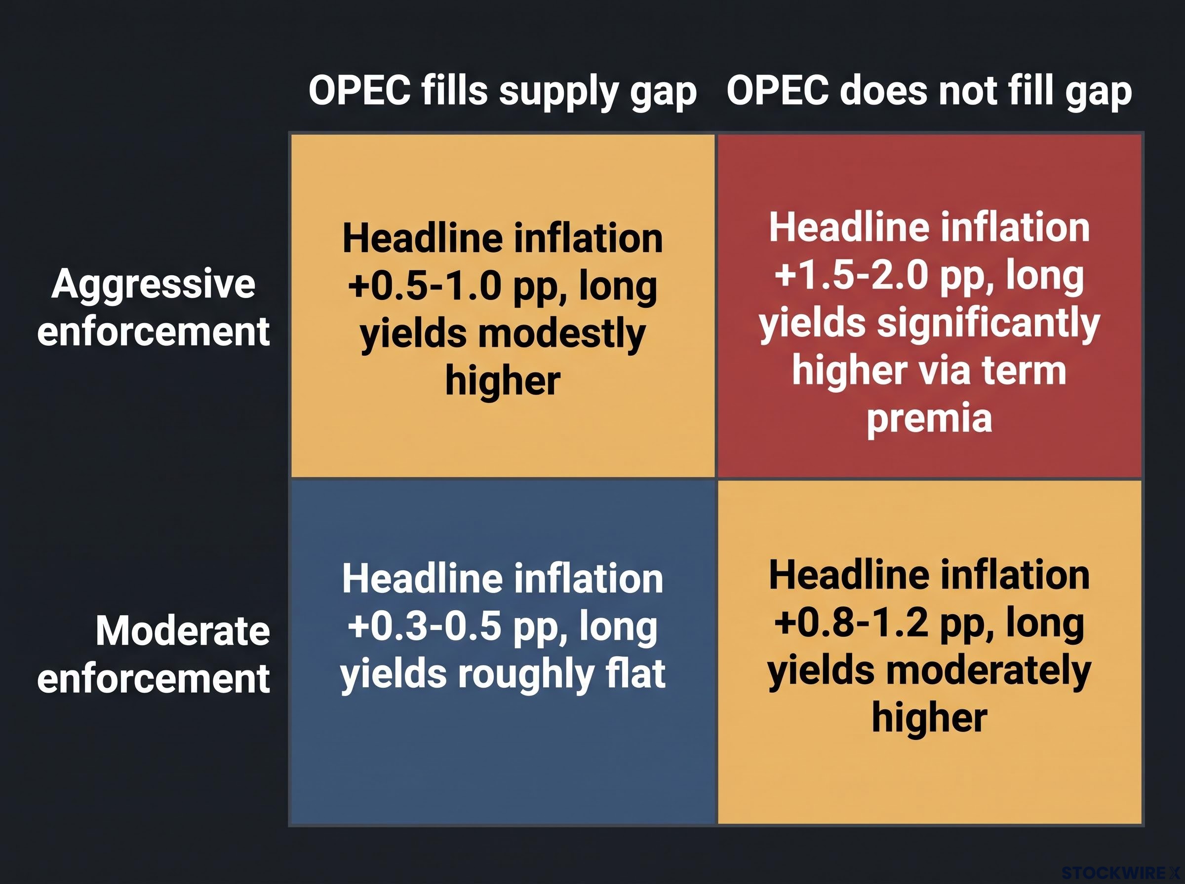
| Enforcement level | OPEC fills supply gap | OPEC does not fill gap |
|---|---|---|
| Aggressive enforcement | Headline inflation +0.5-1.0 pp; long yields modestly higher | Headline inflation +1.5-2.0 pp; long yields significantly higher via term premia |
| Moderate enforcement | Headline inflation +0.3-0.5 pp; long yields roughly flat | Headline inflation +0.8-1.2 pp; long yields moderately higher |
For bond investors, the distinction between a supply-driven and demand-driven price spike matters directly. Supply shocks show up as higher inflation risk premia in long maturities because markets cannot price in a quick resolution. That persistence is what makes this relevant to term premia specifically, not just the short end of the curve.
Two tools pulling in opposite directions: the net yield outlook for September through November
The core tension is now visible. Buybacks and TGA drawdowns create a known, bounded technical bid on the long end. Iran sanctions create an unbounded fat right tail of inflation risk. These are not two stories. They are one story about asymmetry.
The distribution of long-yield outcomes over the 9 September to 4 November window is not symmetrical. On one side sits modest, fairly predictable downward technical pressure: approximately $83 billion in maximum long-end repurchases, material at the margin but small relative to a $32 trillion market. On the other side sits a larger but conditional upward shock driven by the sanctions-oil-inflation channel.
The net outlook is a skewed distribution: modest and knowable downward technical pressure from buybacks versus a fat right tail driven by the sanctions-oil-inflation channel.
For a bond investor positioned in long-duration Treasuries, the buyback programme provides a floor that is real but thin. The sanctions-oil-inflation channel represents a ceiling risk that is conditional but potentially large. Sizing that asymmetry is the practical decision this analysis enables.
Three variables determine which force dominates:
- Pace and composition of TGA drawdown relative to bill issuance: If the TGA is drawn down without proportional bill issuance, shadow easing supports the long end; if bill issuance offsets, the liquidity injection is muted
- Enforcement intensity of Iran secondary sanctions and tanker traffic data through the Strait of Hormuz: Aggressive enforcement with further traffic deterioration signals the inflationary tail is materialising
- OPEC production response in the weeks following the sanctions announcement: If other producers fill lost barrels, the inflation channel weakens; if spare capacity stays sidelined, the fat right tail grows fatter
Neither complacency nor panic is warranted. Treating the buybacks as a reliable lid on long yields ignores the sanctions channel. Treating the sanctions as a guaranteed blow-out ignores the technical bid and the scenario dependency. The asymmetric framing gives you a structure for updating your view as new data arrives, rather than a point prediction that expires.
Reading the macro plumbing: three indicators to watch through November
The analytical structure above converts into three leading indicators you can monitor before yield moves are fully priced:
- TGA balance trajectory: Currently at approximately $950 billion. A sustained drawdown signals reserve injection and supports risk assets; a flat or rising balance signals continued shadow tightening.
- Track via the daily Fed H.4.1 statistical release, which reports the TGA balance
- Strait of Hormuz vessel traffic: Currently at approximately one-fifth of pre-conflict levels. Further deterioration signals that sanctions enforcement is biting harder than expected; partial recovery signals supply normalisation.
- Track via vessel-tracking services such as MarineTraffic or Kpler tanker flow data
- OPEC production response: Saudi, UAE, and broader OPEC+ production announcements in the weeks following 24 August will signal whether lost Iranian barrels are being replaced.
- Track via IEA monthly oil market reports and OPEC+ communiqués
These indicators are leading, not lagging. If you track them in combination, you have a materially better framework for anticipating long-yield direction than if you rely on Fed meeting calendars alone. Over this particular window, the dominant forces are fiscal and geopolitical, not monetary.
The Fed H.4.1 statistical release reports the TGA balance alongside reserve balances and other factors affecting the Fed’s balance sheet, making it the primary data source for tracking whether drawdowns are translating into the reserve injections the shadow-easing thesis depends on.
Which force wins depends on a variable the administration controls
The most uncomfortable feature of this situation is that the same policy apparatus is pulling in both directions. The administration can modulate how aggressively it pursues secondary sanctions, which means the inflationary tail is partially endogenous to the same Treasury building that is simultaneously running the buyback programme.
That internal tension is unlikely to resolve cleanly. Bond markets will price the uncertainty itself as a risk premium, even before any oil shock fully materialises. Iran’s national security chief calling the measures “an act of war” is a signal that escalation risk is not a tail scenario; it is a live variable.
The net characterisation: modest, knowable downward technical pressure from the buyback programme versus a fat right tail driven by the sanctions-oil-inflation channel. The distribution is skewed, and the key branching variable, enforcement severity, is a policy choice.
The buyback ceiling of $4 billion minimum per operation, translating to approximately $83 billion maximum for the window, is a real but thin technical support. Whether it matters depends on whether sanctions enforcement is dialled to a level that triggers a genuine oil shock, pushing headline inflation by an estimated 0.5-2 percentage points and embedding a durable risk premium in long-term yields.
For investors wanting to examine the confidence problem behind the programme’s limits, our deep-dive into why the buyback failed to hold the long end documents the intraday reversal pattern and the four structural forces, rising real term premia, fiscal supply, persistent inflation, and competing corporate issuance, that overwhelmed the technical bid.
The key risk to a long-duration Treasury position over the next two months is not monetary policy. It is an enforcement decision made in the same building that runs the buyback programme. That distinction changes what you should monitor and how you should hedge. When new information arrives about sanctions enforcement or OPEC production response, you know exactly how to update your view: check whether the inflationary tail is growing or shrinking, and size your duration exposure accordingly.
This article is for informational purposes only and should not be considered financial advice. Investors should conduct their own research and consult with financial professionals before making investment decisions. Financial projections and scenario estimates referenced are subject to market conditions and geopolitical developments that may change rapidly.